Original solutions to both sections, all six questions and all twenty-nine terminal parts of the Numerical Linear Algebra and Continuous Optimisation paper sat on 8 June 2010. Source: released Mathematics papers,
Part C 2007 11.pdf. Statements are not reproduced.An orthogonal projector sends to the foot of its perpendicular onto the image of a linear map . The residual is orthogonal to the entire range, not just to the single vector . Indeed, for any range vector ,In particular . The orthogonal projection diagram illustrates the resulting right triangle.
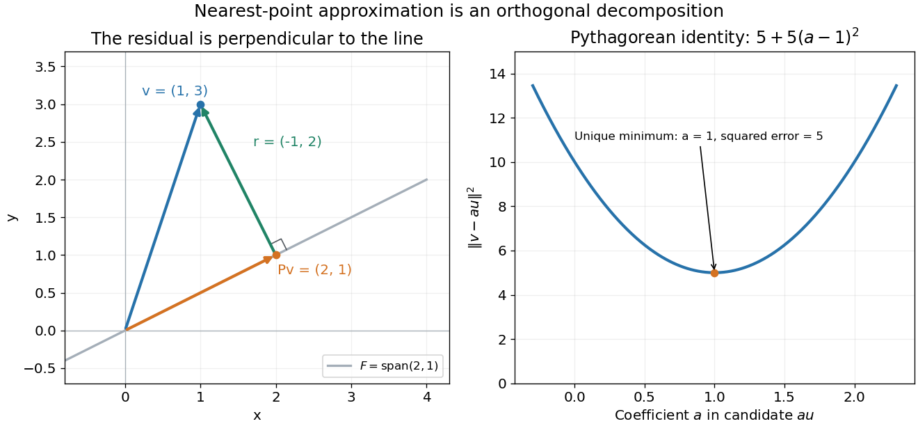
An orthogonal projector maps a vector to its perpendicular foot on the range; the residual is orthogonal to that range
. Details. 
The vector Euclidean norm is , the ordinary length from the origin. The induced matrix norm isGeometrically this is the largest stretch of a unit vector. A linear map sends the unit sphere to an ellipsoid, possibly degenerate; its largest semiaxis has length . Equivalently the matrix 2-norm is the largest singular value.
The perpendicular decomposition in part (a) gives, by the Pythagorean theorem,Thus an orthogonal projection cannot lengthen a vector and . Algebraically the cross term vanishes because , giving the same identity directly from the hypotheses. If , take a nonzero in its range; then and . For the norm is zero.
The nullspace is the vector subspace . A full real singular value decomposition iswhere are orthogonal matrices and for , with for . We may order . The columns of form an orthonormal basis of the input space , and the columns of form one of the output space . The positive singular values number exactly the matrix rank.
Let be the matrix rank, and partition the right singular vectors as , with consisting of the columns associated with zero singular values. From , these columns form an orthonormal basis of the nullspace. Therefore its orthogonal projector isIt acts on the input space . Symmetry and idempotence follow from . At full column rank it is zero, and at rank zero it is the identity.
At elimination column , let be the size of the remaining trailing block. Computing its multipliers costs divisions; updating all entries costs floating-point operations, one multiplication and one subtraction per entry. Thus the dominant count isUpdating the right side and back substitution add only floating-point operations. Pivot searches involve comparisons and row exchanges, without changing the leading arithmetic count. Hence Gaussian elimination with pivoting has the requested asymptotic cost.
An orthogonal similarity transformation is with . An upper Hessenberg matrix has whenever ; its first subdiagonal may be nonzero.
At step , choose a Householder reflector whose trailing block sends the current column segment in rows to a multiple of its first coordinate. The left multiplication zeros positions . Apply the matching right multiplication to retain similarity: . Since acts only on rows and columns , earlier Hessenberg zeros are preserved. Finally gives .
Each reflector is applied through a rank-one update, costing rather than a full matrix multiplication. Across steps, the Hessenberg reduction costs .
Solving the unrelated shifted systems by separate Gaussian elimination costs floating-point operations.
Instead compute once in work. For each shift, solveThe shift changes only the diagonal, so remains an upper Hessenberg matrix. In each elimination column only the entry immediately below the pivot needs removal. With partial pivoting the only possible nonzero candidate rows are the current row and the next, and each update touches entries. Factorization therefore costs per shift; the triangular solve and both orthogonal-vector transformations also cost each.
Thus shifted solves plus the initial Hessenberg reduction cost in total. Pivoting is still needed in general: nonsingularity excludes a singular system but does not by itself guarantee that every unpivoted elimination pivot is nonzero.
The off-diagonal Toeplitz matrix is symmetric and has row and column absolute sums bounded byFor an elementary Euclidean bound, apply the weighted Cauchy-Schwarz inequality in each row:Sum over and use both absolute-sum bounds to get . ThereforeThe entry is unused because the diagonal of is fixed to one; including it only weakens the bound. This is the row-column bound for the matrix 2-norm.
A real symmetric matrix is positive-definite when for every nonzero real vector . The preceding matrix 2-norm bound givesThus is a symmetric positive-definite matrix, independently of the detailed positions of the nonzero entries of .
An eigenvalue of is a scalar for which has a nonzero eigenvector. Allowing initially , symmetry of the real matrix gives , so is real. Since ,This proves reality without presuming it when choosing the eigenvector. Once is real, the real or imaginary part of supplies a nonzero real eigenvector.
For a unit eigenvector of , . The matrix 2-norm bound from part (a) gives . Hence every eigenvalue lies inIn particular the condition number in the Euclidean operator norm satisfies .
The energy norm associated with this symmetric positive-definite matrix isIt is the norm induced by the inner product . The conjugate gradient method minimizes this error norm over its successive affine Krylov subspaces.
The standard conjugate gradient convergence bound isHere , so the factor in parentheses is at most . Since , 25 iterations suffice to reduce the energy-norm error by a factor exceeding .
There are at most nonzero entries of , and each contributes to at most two off-diagonals. Thus has at most nonzero entries. Initialize a matrix-vector product with the diagonal contribution , which costs no arithmetic because the diagonal is one. Each off-diagonal term needs one multiplication and one addition, giving at most floating-point operations per product.
A standard conjugate gradient step adds two inner products, three vector updates and two scalar divisions, at most further operations. Starting from makes and avoids an initial matrix-vector product; its squared norm needs operations. The total for 25 steps is at mostThis supplies an explicit meaning of the paper's large- qualification. The quoted conjugate gradient convergence bound is the usual exact-arithmetic result.
At an unconstrained local minimizer of a twice continuously differentiable objective function, the first-order optimality condition is . The second-order necessary condition is for every direction , so the Hessian matrix is positive semidefinite.
For the Euclidean norm, the unit steepest descent direction is when ; the algorithm usually uses the unnormalized direction . It is a descent direction because .
Two limitations of unpreconditioned steepest descent method in high-accuracy smooth optimization are its slow zigzagging on ill-conditioned valleys and its sensitivity to scaling of the coordinates. It uses no curvature information to correct those directions, so it can require many function and gradient evaluations compared with a suitable Newton or quasi-Newton method. These are reasons to prefer curvature-aware methods in that setting, rather than a claim that gradient-based methods are never useful.
The descent lemma follows by integrating the gradient along the line and using its Lipschitz continuity:This upper bound is at most the right side of the Armijo condition when . Since , it holds forThe zero step gives equality; every positive step in this interval satisfies the prescribed sufficient-decrease test.
The quadratic model has gradient and positive-definite Hessian matrix . Its unique minimizer is thereforeIf , then and , proving that it is a descent direction.
Backtracking line search starts with a trial step and repeatedly reduces it until the Armijo condition holds. Part (ii) guarantees finite termination because sufficiently small steps are acceptable. The test guarantees a specified positive fraction of the decrease predicted by the linear model, namely for an accepted positive step. It does not require solving the line-minimization problem exactly.
If the first trial is accepted, . Otherwise the preceding trial was rejected and so exceeded , since part (ii) guarantees acceptance below that threshold. The accepted step, reduced by the factor , consequently exceeds . In either case,The angle condition gives . Hence the backtracking line search has the lower bound
From and the matrix 2-norm bound, , so . Let . The summand in the supplied decrease bound satisfiesThus, with the fixed positive constant ,The nonnegative series therefore converges, forcing its terms to zero:The argument uses the given angle condition and upper bound on ; it does not need an additional uniform lower eigenvalue bound on .
Use the optimization Lagrangian , with and . Under the usual linear independence constraint qualification, a local minimizer has multipliers satisfying the equality-constrained Karush-Kuhn-Tucker conditionsThe second-order necessary condition isOnly feasible tangent directions enter this last test; the Hessian matrix need not be positive semidefinite on the entire ambient space.
With , differentiation of the quadratic penalty method objective givesThe primal Newton system is thereforeFor bounded multipliers and regular derivatives, remains of ordinary size while becomes large in directions normal to the constraints. If the feasible tangent space is nontrivial and retains ordinary-size curvature, this produces a large condition number as .
Introduce . The same step is obtained from the symmetric augmented systemEliminating recovers the primal system exactly. This matrix contains no explicit entries and tends to a saddle-point matrix. Under full row rank of the limiting constraint Jacobian matrix and nonsingularity of the limiting reduced Hessian, that limiting matrix is nonsingular, so this formulation avoids the artificial penalty-induced separation of scales.
These conditioning statements require regularity beyond bounded alone. A rank-deficient constraint Jacobian matrix or singular reduced Hessian can still make the augmented system ill-conditioned. If and is nonsingular, all directions may scale together in the primal system, so a large condition number is not automatic there either.
Complete the square in the augmented Lagrangian method objective:For fixed , the last term is constant in . Thus its minimization is the quadratic penalty method applied to the shifted constraint .
Its practical advantage is that multiplier updates, typically , can drive the original constraint residual to zero while stays moderately sized. The plain quadratic penalty method generally needs very small to produce the same feasibility accuracy, exposing the conditioning problem in part (ii).
The linearized constraints may be inconsistent, for example when is not in the image of a linear map defined by . Even if feasible, the quadratic objective may have negative curvature along its feasible tangent space, making it unbounded below and leaving no local minimizer.
Fletcher's Sℓ1QP replaces the hard linearized constraints by an L1 exact penalty and bounds the step inside a trust region. One usual form isThe zero step is always admissible. The trust region is compact, so a minimum exists even when the model Hessian matrix is indefinite; the constraint penalty measures infeasibility rather than making the subproblem impossible to solve. Adjusting its weight promotes feasibility, while the radius keeps the local model within a controlled neighbourhood. Introducing nonnegative positive- and negative-part slack variables converts the absolute values to an equivalent smooth quadratic program with box constraints.[ref]
Sequential Quadratic Programming Methods by Philip E. Gill and Elizabeth Wong. §3.3, equations (3.25)–(3.26): Fletcher's Sℓ1-QP model and its elastic quadratic-program formulation
Stationarity of the equality-constrained quadratic model gives , while feasibility gives . A symmetric system linking the step and new multiplier isLet have columns forming a basis of . The saddle-point matrix is nonsingular exactly when has full row rank and is nonsingular. Full row rank is necessary because a nonzero vector in would give a null vector of the block matrix. Under full row rank, solving a homogeneous system forces and then ; this proves sufficiency and the converse. Positive definiteness of the reduced Hessian is sufficient for a constrained minimum but is stronger than the nonsingularity condition asked here.
A null-space method first finds with , then solvesand recovers from . It needs the stated full row rank and nonsingular reduced matrix; Cholesky decomposition is available when the latter is positive definite.
A range-space method additionally assumes is invertible. It solves the Schur complement equationsIf is positive definite and has full row rank, the Schur matrix is positive definite and both solves can use Cholesky decomposition. An indefinite but invertible instead requires a suitable indefinite factorization; the Schur matrix must remain nonsingular.
For , the inequality-constrained Karush-Kuhn-Tucker conditions areUnder an appropriate constraint qualification, the second-order necessary condition is on the critical coneEquivalently active constraints with positive multiplier require , while active zero-multiplier constraints retain . Inactive constraints impose no first-order tangent restriction. This distinction is why the relevant cone need not be the nullspace of every active row.
On the strictly feasible region , the logarithmic barrier objective isWith , its gradient isThe positive coefficients are the barrier's multiplier estimates.
The equation , together with and , is the perturbed Karush-Kuhn-Tucker conditions: stationarity is unchanged, while exact complementary slackness becomes for each . A finite limit of such points as satisfies the original conditions by continuity.
For a strictly feasible , the second block uniquely specifies . Substitution into the first block gives precisely . Thuswithin the stated strictly positive domain. These are stationary barrier points; they need not all be local minimizers in a nonconvex problem.
The Jacobian matrix of in isThe top-left block is the Hessian matrix of with held fixed. In the second block, differentiating in gives and in gives . The explicit derivative with respect to is . Differentiate by the chain rule:All blocks are evaluated on the current central path point.
At the current exact path point , stationarity is already zero and . Therefore . Its Newton correction solvesThe matrix has no explicit dependence on the barrier parameter, so comparison with part (iv) giveswhen is nonsingular. If it is singular, the displayed vector is still a solution of the correction equations, but uniqueness of the correction cannot be inferred from differentiability of the path alone.
This step is exactly the tangent predictor in the stated first-order Taylor expansion. For nearby positive , it approximates the new path point with error ; a bounded second path derivative improves this to . Continuity also preserves strict positivity for sufficiently small parameter changes. Larger changes may require damping to keep both the constraint values and multiplier estimates positive.
Articles by others on the same topic
There are currently no matching articles.