For independent Gaussian measurements with correctly specified standard deviations, model residuals give the chi-squared test statisticFor a linear fit of identifiable parameters under the null model, it has a chi-squared distribution with degrees of freedom. The upper-tail p-value tests unusually large residuals; a nonlinear fit generally uses this distribution only approximately. Correlated Gaussian errors instead require .
For counts, Pearson's chi-squared test uses , with calculated under the null hypothesis. For multinomial categories and fitted parameters the usual asymptotic degrees of freedom are ; the subtraction of one reflects the fixed total count. Sparse expected counts can invalidate this approximation, requiring a suitable exact or simulation-based test. Contingency-table independence gives degrees of freedom.
A small p-value indicates tension with the specified model and error assumptions; it is not the probability that the null is true. Excessive may reflect a wrong model, underestimated errors, correlations or outliers. An implausibly small value may suggest overestimated errors or hidden constraints. For an adequate fitted model is typically near one, with fluctuations, rather than required to equal one.
Measure an unwanted effect separately or design a comparison in which it cancels. Calibration against reference standards at several settings tests zero offset, gain and nonlinearity. Blanks reveal background. Reversal is useful when the wanted response is odd and the nuisance is even: gives and . For example reversing current in a resistance measurement cancels a stable thermoelectric voltage, but does not cancel the current-scale error or even-in-current Joule heating.
Interleave reversals to detect drift; interchange sensors or leads to expose asymmetry. Null or bridge methods reduce dependence on detector gain. Alignment checks, shielding and temperature control target specified physical couplings. Independent measurement methods provide a stronger test than repetition of the same setup. Repeated readings reduce independent random errors, not a shared bias. Correct significant identified effects and propagate the uncertainty of the correction and standards; complete removal of an unknown systematic error cannot generally be certified.[ref]
Guidelines for Evaluating and Expressing the Uncertainty of NIST Measurement Results by Barry N. Taylor and Chris E. Kuyatt. §5.2, uncertainty remaining after systematic-effect corrections
Use an enclosure with thermal insulation and sufficient heat capacity to slow the response to ambient changes. Block draughts and direct radiant heating, use low-conductance supports and thermal breaks in wiring, and reduce thermal radiation with low-emissivity shields. Vacuum suppresses gas thermal conduction and convection but leaves thermal radiation and solid thermal conduction. A conducting inner shield helps make temperature uniform; it is not by itself thermal insulation.
For a lumped load of heat capacity coupled to the room by thermal conductance , the first-order thermal isolation model isLarge thermal resistance and heat capacity attenuate fast fluctuations; nested shields can provide several filtering stages. Passive thermal insulation does not reject arbitrarily slow ambient drift, since this transfer approaches one at zero frequency. It also increases the temperature rise caused by internal dissipation.
For long-term stability use a regulated bath or thermostat, placing a calibrated sensor near the sensitive component. Heater feedback rejects slow disturbances, provided sensor lag, loop stability, actuator range and electrical pickup are controlled. Maintain stable internal power, allow equilibration, record both room and load temperatures, and test rejection by a deliberate ambient-temperature step or sinusoidal modulation. These measurements reveal gradients and thermal bypasses that an thermal insulation label alone cannot establish.
An ideal operational amplifier has infinite input impedance and open-loop gain, zero output impedance and no offsets or response limits. Its input currents vanish. Stable operational-amplifier negative feedback, a finite output and unsaturated linear operation then imply a virtual short, . Real amplifiers have finite frequency-dependent gain, input bias currents, offset voltage, output loading, finite bandwidth, slew rate and supply-rail limits. Equal input voltages cannot be assumed in an open-loop or saturated circuit.
Here the noninverting input is grounded. In the ideal-feedback limit the inverting node is a virtual ground, so the resistor current charges the feedback capacitor:The initial capacitor charge fixes the integration constant. This is an op amp integrator, with .
A tiny direct-current input, input bias current or offset can drive the output towards saturation. A parallel feedback resistor provides a direct-current return path, giving ; choose over the intended integration band. A reset switch sets initial charge; low-offset components and suitable signal amplitude reduce drift and saturation. The useful band must also remain below the amplifier's bandwidth and slew-rate limits.
For the stipulated finite but constant real gain , infinite input impedance and negligible output impedance, write the inverting-node voltage as . With phasors proportional to ,ThereforeThe low-frequency gain is . The corner is ; above it the amplitude falls as and the phase approaches . phase and describe the same low-frequency inversion. This finite-gain circuit is a low-pass response with an integrating high-frequency regime, not an ideal integrator down to zero frequency. A genuinely frequency-dependent would introduce additional high-frequency limitations beyond this specified model.
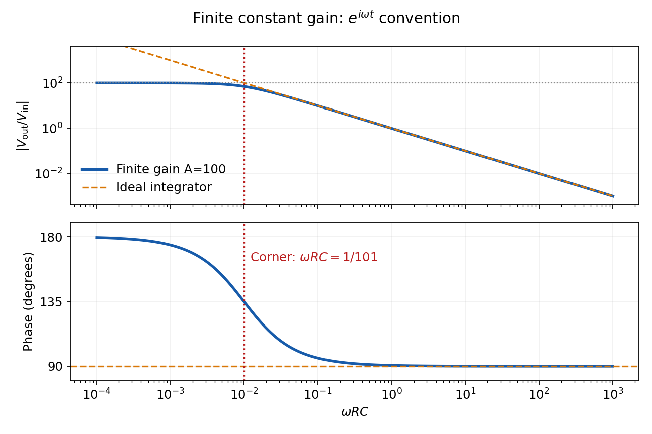
Finite-gain integrator response
. Details. 
Articles by others on the same topic
There are currently no matching articles.