Original paper: FOI release, physical PDF pages 8–13, printed pages 1–6. Every optional question and note topic is answered.
As an estimate, model the confinement by an infinite square well of width and use the stipulated electron mass. Its energy eigenvalues are , , so the gap controlling thermal occupation of a quantum well isThus suppresses excitation: . For example makes this ratio below one percent in this model. There is no sharp cutoff. The ground state energy itself corresponds to about , but it is the excitation gap that enters the Boltzmann factor. Finite barrier height and a different effective mass would change the numerical scale; neither is supplied.
For normalized amplitudes and a time-independent observable , the Schrödinger equation givesThe interference term therefore hasThis is the period of two-state quantum interference. If the off-diagonal matrix element or either amplitude vanishes, the expectation value is constant, so this is not its unique fundamental period. Equal energies likewise give no beat.
The Sturm oscillation theorem requires respectively zero, one and two nodes of a wavefunction. Treating the vertical outer boundaries as hard walls, all three wavefunctions vanish there. The potential energy is asymmetric, so no even/odd parity should be imposed. At internal finite steps, both the wavefunction and its first derivative are continuous.
For and , only the left well is classically allowed. Their wavefunctions oscillate there and continue as evanescent combinations through the barrier and right region, reaching zero at the far wall. The first is nodeless; the second has one node in the left well. For both wells are allowed, while the central barrier remains forbidden: the wavefunction oscillates in both wells, with an evanescent bridge and two nodes of a wavefunction overall. A node may lie inside a finite forbidden barrier when the matching coefficients have opposite signs. Precise node positions and relative amplitudes require dimensions and heights not specified by the qualitative drawing.
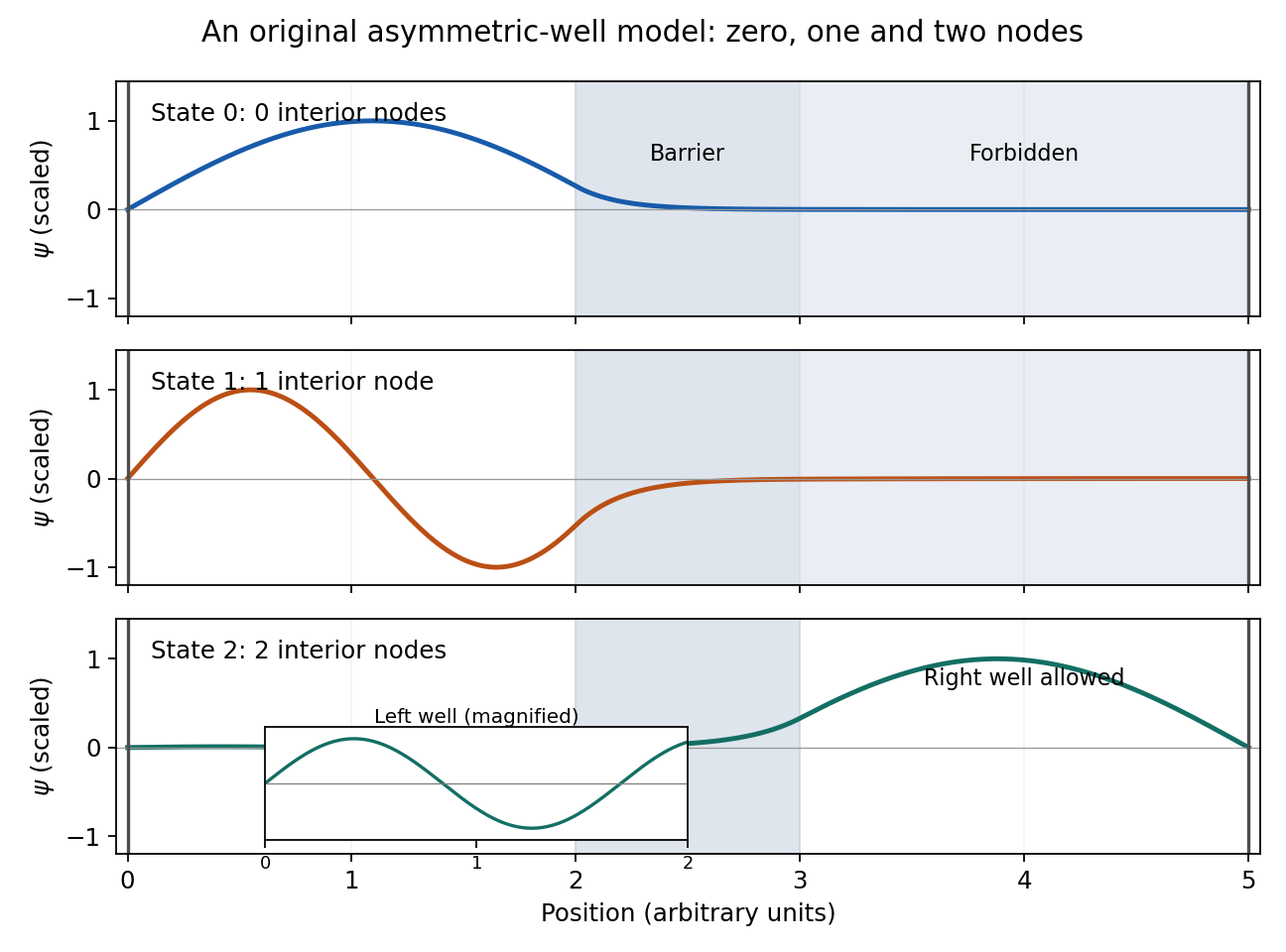

The original illustration solves an explicitly chosen model with the same ordering of allowed and forbidden regions. Its numerical parameters and detailed node positions are illustrative.
Assuming independent Gaussian measurement errors with the quoted standard deviations, use the inverse-variance weighted mean:Here and , givingThe consistency statistic is for four degrees of freedom, so there is no evident excess scatter requiring error rescaling. A shared systematic error would require a covariance matrix and would not be reduced by this averaging rule.
A small constant input can repeatedly produce the same analogue-to-digital converter code, so averaging those codes cannot reveal its position within a conversion interval. dither makes adjacent codes toggle; their relative frequencies then encode changes smaller than one conversion step. With adequate oversampling, low-pass filtering and averaging reduce the added, sufficiently uncorrelated noise while retaining the slow signal.
For independent sample errors, the averaged standard deviation scales as ; ideally four times as many samples gain about one effective bit. For example a constant input rounded to levels separated by would always return zero. Adding uniform dither on gives output with probability and zero otherwise: the expected average is , with error . The benefit concerns the filtered estimate, not a more accurate individual conversion. Excessive dither wastes range, and averaging does not correct calibration bias, correlated drift or arbitrary converter nonlinearity.[ref]
AN-1549: Performance Optimization of the Integrated ADC on the ADuCM4050 by Analog Devices. Oversampling and Averaging, especially the dither and uncorrelated-noise discussion; Table 1
The parity operator acts as , with . For an even potential energy , so energy eigenstates can be chosen even or odd, with parity eigenvalues and . One-dimensional bound states are nondegenerate; the ground state is nodeless and even.
For the finite square well, square integrability excludes the growing exterior exponential, while even parity excludes the interior sine. Thus the interior solution is proportional to , with matching decaying tails andContinuity at gives and . Their ratio yieldsThe conditions at follow from the same parity.
For a narrow weak well, , hence andThis is self-consistent because . It is the shallow finite-square-well energy, equivalently the attractive delta potential limit with integrated strength . An arbitrarily weak attractive well of this form still has its even bound ground state.
The first excited state must be odd. Replace the interior cosine by and choose exterior tails with opposite signs. The matching condition becomes . Its first root requires . At the binding threshold , sois necessary and sufficient for the first odd bound state. Equality gives a zero-energy nonnormalizable threshold solution, not an additional bound state.
Writing , where and , the canonical commutation relation givesConsequently and . If were nonzero, this commutator would make it an energy eigenstate with energy , contradicting the lowest-energy property. Therefore .
The commutator product rule and induction giveActing on the vacuum and shifting the sum then shows that the unnormalized bosonic coherent state satisfies .
The displayed series lacks its wavefunction normalization factor. Since , its squared norm is . The normalized coherent state needed for the stated expectation values isUse , , and . For , ,The displacement changes the mean position but not its ground-state uncertainty. Unnormalized bras and kets give the same physical expectation values only after division by their squared norm.
The angular-momentum commutators giveFor example . In the displayed basis , the only nonzero upper entries of connect adjacent magnetic quantum numbers. Subtracting their column and row eigenvalues multiplies each by , proving the first matrix commutator; the lower matrix similarly gives the second. Direct multiplication giveswhose difference is . Also , confirming .
A rotation changes the quantization axis without changing the spectrum, so has eigenvalues . Its dimensionless matrix isSolving and normalizing gives the spin-one maximum-projection eigenvectorFor instance the first equation is , and the squared components sum to one. An overall phase is immaterial.
At , . The Born rule therefore predicts, in the requested order,This treats the Stern-Gerlach experiment as the stipulated ideal measurement of orbital projection. In an actual atom, other magnetic moments and spin-orbit coupling can change which angular momentum the apparatus resolves.
With angular-coordinate measure , the normalized one-particle orbitals are . Single-valuedness requires integer . Their products obeyIf arc-length measure is used instead, each one-particle wavefunction normalization includes ; the physical energy is unchanged. For the following parts impose antisymmetry on the full spatial-and-spin state of the two fermions.
Both particles can occupy with opposite spins, giving a unique singlet state at , quantum degeneracy 1. At the next distinct energy , one orbital is and the other is or . For each orbital choice there is one symmetric spatial state paired with the singlet state, and one antisymmetric spatial state paired with three triplet state spin projections. HenceSwapping particle labels adds no independent state after the required exchange symmetry is imposed.
The lowest singlet state isFor the lowest triplet states take and :orthogonality of and verifies wavefunction normalization of the antisymmetric spatial factor. At this same energy there are also two excited singlet states, obtained by replacing its minus sign with a plus sign and the spin factor by . Together they reproduce the eight states counted in part a.
At coincidence , the triplet state spatial factor vanishes, while the lowest singlet state has finite, uniform pair probability. Consequently a weak short-range repulsion raises the singlet state energy more strongly: antisymmetry suppresses close encounters in the triplet state. In the contact-interaction limit the triplet state contribution is exactly zero, whereas the singlet state shift is positive. A finite-range interaction gives a nonzero but suppressed triplet state shift. This explains a relative energy increase; it does not by itself establish a crossing or justify using unchanged noninteracting wavefunctions for arbitrarily strong repulsion.
For a time-independent Hamiltonian operator, a symmetry operator satisfies , or . Thus applying to an energy eigenstate preserves its energy. Commuting Hermitian observables can be diagonalized within each degenerate energy eigenspace, allowing states to be labelled by symmetry quantum numbers.
A continuous unitary symmetry has Hermitian generator . Differentiating the invariance condition gives . The Heisenberg equation of motion then yieldswhen has no explicit time dependence. spatial translations connect to momentum conservation, rotations to angular-momentum conservation, and time-translation invariance to energy conservation. A central potential energy conserves all components of angular momentum, but they cannot all be assigned sharp simultaneous values because they do not commute; are a compatible choice. Discrete reflection symmetry gives parity labels without a continuously variable generator. A quantum degeneracy can be protected by a symmetry, but a quantum degeneracy alone does not identify its physical origin.
In Compton scattering, a photon transfers energy and momentum to an initially stationary, approximately free electron. With incident and scattered wavelengths and photon deflection angle , momentum conservation givesCombine this with to obtainThe photon loses energy to electron recoil; the shift is independent of incident wavelength in this free-electron model and is largest at backscattering. At energies comparable with atomic binding, initial electron motion, binding and coherent scattering from the atom require additional treatment. Classical elastic scattering from a fixed charge alone does not produce this recoil wavelength shift.
In Arthur Holly Compton's spectral test, molybdenum-target X-rays scattered from graphite at were compared with the primary spectrum using the same slits, crystal and tube potential energy. A calcite crystal resolved the shifted line by Bragg's law; lines on both sides established angular zero. The crystal glancing angle on the plotted axis differs from the photon scattering angle. The compared curves had different intensity scales, and the paper did not directly observe the recoil electrons in this X-ray test. These controls support the wavelength comparison without converting it into a direct recoil-track measurement.[ref]
A Quantum Theory of the Scattering of X-rays by Light Elements by Arthur Holly Compton. pp. 494–496, Experimental Test, Fig. 4 and opening of Velocity of recoil of the scattering electrons
For independent angular momenta , set . Since different subsystems commute, satisfies the same angular-momentum algebra. The product basis diagonalizes ; the coupled basis diagonalizes . Its labels obeyThe Clebsch-Gordan coefficients are the unitary change of basis between them. Start from the maximum-weight state , apply with wavefunction normalization, and construct the remaining multiplets by orthogonality.
For two spin-one-half systems, the symmetric triplet state is , , , with ; the antisymmetric singlet state has . The dimension identity checks completeness. Coupling orbital and intrinsic spin similarly gives total atomic angular momentum and organizes spin-orbit energy splittings. Exchange symmetry is an additional restriction when the constituents are identical.
quantum tunnelling is transmission through a finite region in which the classical kinetic energy is negative. The wavefunction need not vanish there: the Schrödinger equation permits evanescent solutions. The transmitted particle retains its conserved energy; it does not borrow energy to surmount the barrier.
For a rectangular barrier of height on , with and zero exterior potential energy, define and . A left-incident scattering solution has the three piecesContinuity of at both boundaries imposesEliminating givesEqual incident and exit velocities justify ; different exterior potential energies require the velocity ratio. Probability-current conservation gives . Although either real exponential alone has zero current, their complex-coefficient combination can carry the current crossing the barrier.
For , . A slowly varying barrier generalizes this to the WKB approximation , with matching prefactors and turning-point limitations. This exponential sensitivity explains why very small geometric or energy changes can produce large changes in a tunnelling rate.
In alpha decay, a quasibound alpha particle penetrates the nuclear Coulomb barrier; penetration probability, attempt frequency and nuclear preformation determine the rate. In a scanning tunnelling microscope, a bias between a conducting tip and sample gives current approximately proportional to . Piezoelectric positioning and constant-current feedback probe surfaces, while vibration isolation and electronic-state dependence limit a purely geometric interpretation. Atomic-scale steps and surface reconstruction were resolved in the original surface-imaging study.[ref]
Surface Studies by Scanning Tunneling Microscopy by Gerd Binnig and others. Abstract and pp. 57–61, atomic-scale surface images
In a Josephson junction, coherent tunnelling of Cooper pairs permits , a phase-dependent supercurrent through a weak link. Thus the same barrier physics explains natural decay and underpins sensitive surface and superconducting devices.For independent Gaussian measurements with correctly specified standard deviations, model residuals give the chi-squared test statisticFor a linear fit of identifiable parameters under the null model, it has a chi-squared distribution with degrees of freedom. The upper-tail p-value tests unusually large residuals; a nonlinear fit generally uses this distribution only approximately. Correlated Gaussian errors instead require .
For counts, Pearson's chi-squared test uses , with calculated under the null hypothesis. For multinomial categories and fitted parameters the usual asymptotic degrees of freedom are ; the subtraction of one reflects the fixed total count. Sparse expected counts can invalidate this approximation, requiring a suitable exact or simulation-based test. Contingency-table independence gives degrees of freedom.
A small p-value indicates tension with the specified model and error assumptions; it is not the probability that the null is true. Excessive may reflect a wrong model, underestimated errors, correlations or outliers. An implausibly small value may suggest overestimated errors or hidden constraints. For an adequate fitted model is typically near one, with fluctuations, rather than required to equal one.
Measure an unwanted effect separately or design a comparison in which it cancels. Calibration against reference standards at several settings tests zero offset, gain and nonlinearity. Blanks reveal background. Reversal is useful when the wanted response is odd and the nuisance is even: gives and . For example reversing current in a resistance measurement cancels a stable thermoelectric voltage, but does not cancel the current-scale error or even-in-current Joule heating.
Interleave reversals to detect drift; interchange sensors or leads to expose asymmetry. Null or bridge methods reduce dependence on detector gain. Alignment checks, shielding and temperature control target specified physical couplings. Independent measurement methods provide a stronger test than repetition of the same setup. Repeated readings reduce independent random errors, not a shared bias. Correct significant identified effects and propagate the uncertainty of the correction and standards; complete removal of an unknown systematic error cannot generally be certified.[ref]
Guidelines for Evaluating and Expressing the Uncertainty of NIST Measurement Results by Barry N. Taylor and Chris E. Kuyatt. §5.2, uncertainty remaining after systematic-effect corrections
Use an enclosure with thermal insulation and sufficient heat capacity to slow the response to ambient changes. Block draughts and direct radiant heating, use low-conductance supports and thermal breaks in wiring, and reduce thermal radiation with low-emissivity shields. Vacuum suppresses gas thermal conduction and convection but leaves thermal radiation and solid thermal conduction. A conducting inner shield helps make temperature uniform; it is not by itself thermal insulation.
For a lumped load of heat capacity coupled to the room by thermal conductance , the first-order thermal isolation model isLarge thermal resistance and heat capacity attenuate fast fluctuations; nested shields can provide several filtering stages. Passive thermal insulation does not reject arbitrarily slow ambient drift, since this transfer approaches one at zero frequency. It also increases the temperature rise caused by internal dissipation.
For long-term stability use a regulated bath or thermostat, placing a calibrated sensor near the sensitive component. Heater feedback rejects slow disturbances, provided sensor lag, loop stability, actuator range and electrical pickup are controlled. Maintain stable internal power, allow equilibration, record both room and load temperatures, and test rejection by a deliberate ambient-temperature step or sinusoidal modulation. These measurements reveal gradients and thermal bypasses that an thermal insulation label alone cannot establish.
An ideal operational amplifier has infinite input impedance and open-loop gain, zero output impedance and no offsets or response limits. Its input currents vanish. Stable operational-amplifier negative feedback, a finite output and unsaturated linear operation then imply a virtual short, . Real amplifiers have finite frequency-dependent gain, input bias currents, offset voltage, output loading, finite bandwidth, slew rate and supply-rail limits. Equal input voltages cannot be assumed in an open-loop or saturated circuit.
Here the noninverting input is grounded. In the ideal-feedback limit the inverting node is a virtual ground, so the resistor current charges the feedback capacitor:The initial capacitor charge fixes the integration constant. This is an op amp integrator, with .
A tiny direct-current input, input bias current or offset can drive the output towards saturation. A parallel feedback resistor provides a direct-current return path, giving ; choose over the intended integration band. A reset switch sets initial charge; low-offset components and suitable signal amplitude reduce drift and saturation. The useful band must also remain below the amplifier's bandwidth and slew-rate limits.
For the stipulated finite but constant real gain , infinite input impedance and negligible output impedance, write the inverting-node voltage as . With phasors proportional to ,ThereforeThe low-frequency gain is . The corner is ; above it the amplitude falls as and the phase approaches . phase and describe the same low-frequency inversion. This finite-gain circuit is a low-pass response with an integrating high-frequency regime, not an ideal integrator down to zero frequency. A genuinely frequency-dependent would introduce additional high-frequency limitations beyond this specified model.
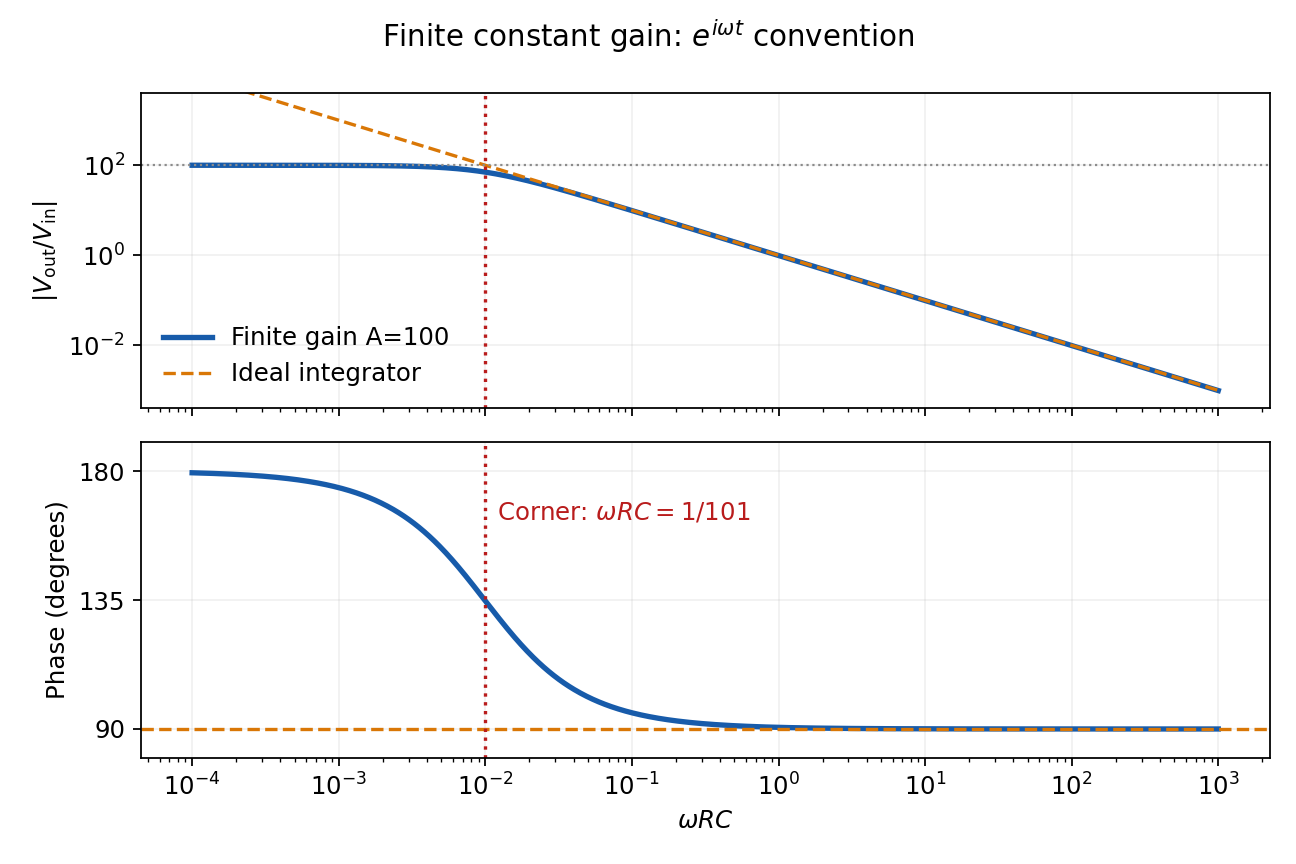
Finite-gain integrator response
. Details. 
Articles by others on the same topic
There are currently no matching articles.