Define and use the independent quoted Gaussian errors , with period and exoplanet transit epoch fixed. The model is linear in despite its sinusoidal time dependence. Minimize . With the normal equations areUsing and , the solution isThe residuals in observation order are . Therefore for degrees of freedom, giving reduced . The upper-tail probability is about : the fit is consistent with the stated errors, although five points do not establish a unique physical explanation.
For known errors the covariance matrix is . Equivalently, profiling out the fitted offset givesThis is the one-parameter uncertainty, not the curvature with incorrectly held fixed. Propagating it through the supplied mass relation, and treating its coefficient and as fixed,The symbol in the exoplanet transit epoch denotes periodic copies of the same exoplanet transit phase, not an uncertainty distribution to propagate. No independent error for the empirical mass coefficient was supplied.
Additional independent observations retain positive weight even with twice the error: each has one quarter of the previous per-observation weight. Their information adds to the existing information matrix, so the formal mass uncertainty decreases for informative additional orbital phases and cannot increase under this fixed-error model. It can remain unchanged in a degenerate phase configuration that supplies no further amplitude information after fitting the offset. The conclusion assumes the same correct model and independent errors, not a new fitted error rescaling or unmodelled systematic effects.
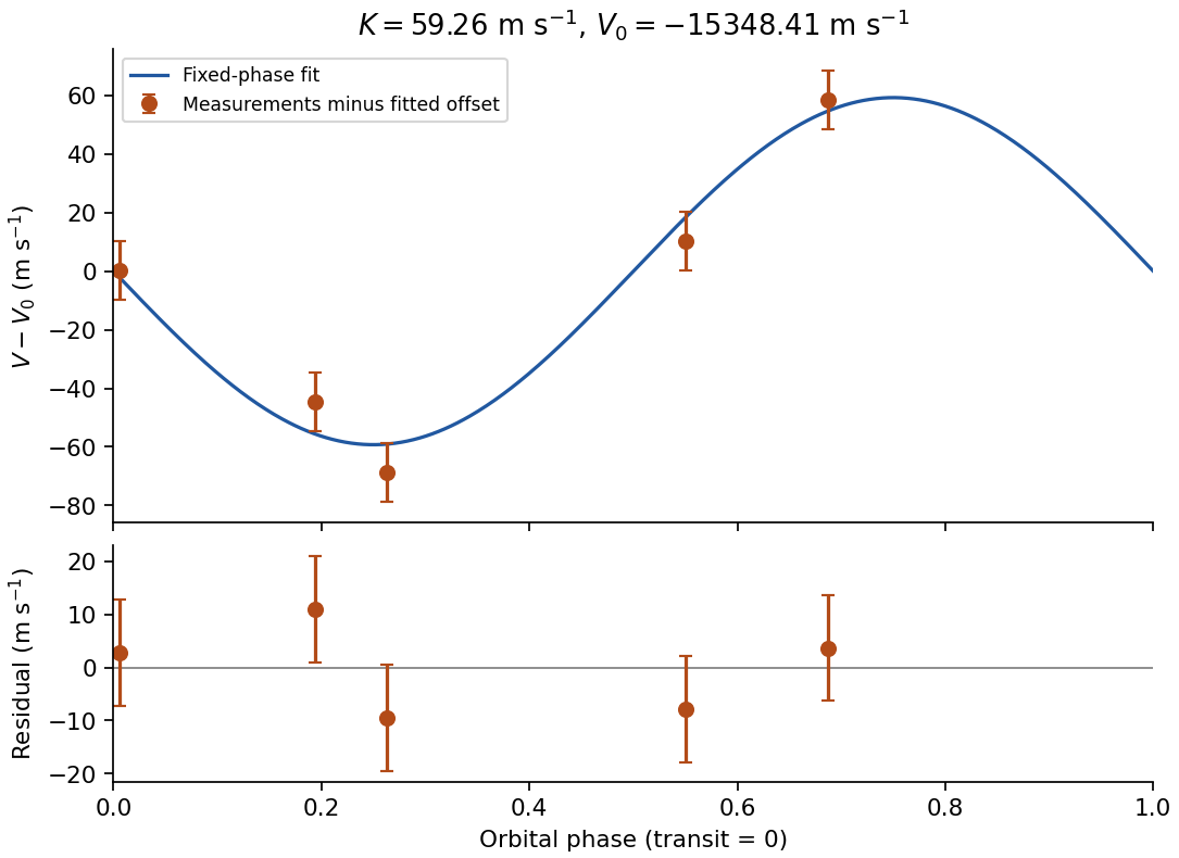
Original plot of the fitted orbital radial-velocity variation and residuals; observed numbers used without reproducing the source table
. Details. 
In an operational-amplifier negative feedback loop, an operational amplifier has large open-loop gain , with . Feeding a fraction back to the inverting input opposes an output increase. For a non-inverting signal input,Its sensitivity to open-loop gain changes is reduced by . Thus resistor ratios can set a reproducible gain despite device variation; feedback also suppresses internal distortion and reduces output impedance. Gain is traded for usable bandwidth, subject to the amplifier's frequency response.
For the non-inverting connection, place between output and inverting input and between that input and ground. Then , giving gain . For an inverting connection, ground the non-inverting input, inject the signal through and return from output to the inverting node. Small differential input and negligible input current then give gain . The near-zero node is a virtual ground, not a physical ground connection.
The feedback must remain stable at the frequencies where loop gain matters. Extra phase lag can turn the intended opposition into oscillation; adequate phase margin, supply headroom, input common-mode range, output-current capability and slew rate are required. Feedback neither prevents clipping nor removes all input noise.[ref]
A lock-in amplifier multiplies the measured signal by a synchronized reference and low-pass filters the product. For and reference , the signal product is . Averaging away the second harmonic gives in this peak-amplitude convention. A second reference gives , soA single quadrature could read zero for a substantial signal from its reference. Two quadratures avoid that blind spot; the phase is undefined at zero amplitude. Instrument RMS calibrations can include a different constant normalization.
The reference shifts the wanted frequency to zero, where a narrow low-pass bandwidth can select it. Uncorrelated broadband noise averages down, whereas a simple amplifier would enlarge signal and noise together. Longer averaging improves narrow-band sensitivity but slows the response to changing amplitude. The signal must remain phase coherent with the reference; frequency mismatch creates a beat instead of a constant output. interference at the same reference frequency survives, so shielding and independent background measurements remain necessary.[ref]
Model SR830 DSP Lock-In Amplifier manual by Stanford Research Systems. printed pp.3-1–3-3, multiplication, dual-phase detection and RMS-versus-peak conventions
Sampling at makes a frequency indistinguishable from , since the extra phase is . For a real sinusoid, reflection to also gives an alias, up to phase. For example, a cosine sampled at has exactly the samples of a cosine. A measured low-frequency feature can therefore originate above the instrument's Nyquist frequency.
To reconstruct an arbitrary baseband signal limited to bandwidth , sample strictly above and use an analogue anti-aliasing filter before the sampler. A practical filter needs a transition band, so merely choosing a nominal rate is insufficient. frequency components already folded together cannot in general be separated by later digital filtering. aliasing from insufficient sampling is distinct from spectral leakage caused by a finite observation window.
Articles by others on the same topic
There are currently no matching articles.