Original solutions to every question and printed alternative. [ref]
https://www.whatdotheyknow.com/request/natural_science_tripos_physics_e_2/response/2340776/attach/2/FOI%202023%20399%20Zahid%20materials.pdf?cookie_passthrough=1#page=86. Original public PDF, physical pages 86–92; dated 24 May 2014
Write the one-electron Coulomb energies as , . The Pauli exclusion principle allows electrons in shell , including spin. The ground configuration therefore has two electrons in and seven in , giving . The least energy-increasing promotion is from to :Rearranging the partly occupied degenerate shell does not produce a higher energy. Both total energies are negative, so this ratio is below one even though .
Choose the centre of the finite square well as the origin and its edges as . The first three bound wavefunctions have even, odd, even parity, with respectively zero, one and two interior nodes. They oscillate inside and decay exponentially outside, with . Both the wavefunction and its first derivative are continuous at each finite potential step. The higher bound states have longer external decay lengths because they lie closer to the barrier height. Overall sign is arbitrary.
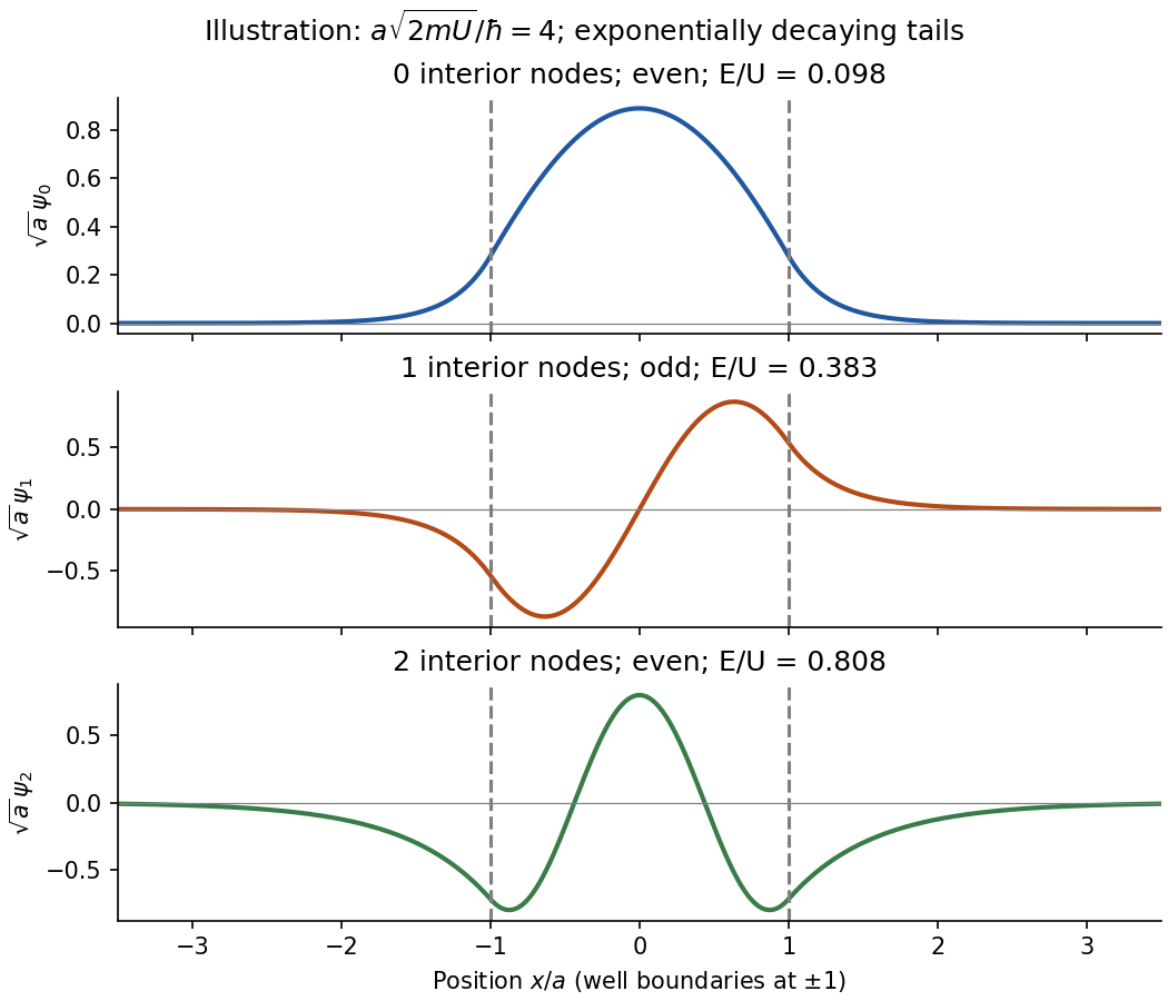
Original normalized finite-well eigenfunctions with parity, nodes and exponential tails; illustrative dimensionless depth, not supplied numerical data
. Details. Confinement to length gives a momentum scale by the Heisenberg uncertainty principle. Using the alpha-particle mass , its speed scale is . Counting encounters with either wall,This is an order-of-magnitude collision-rate estimate, not a classical trajectory of a stationary quantum state. Taking , a different geometric interpretation of the well size, or successive returns to the same wall changes the coefficient by factors of order unity; the robust scale is .
Let denote detection. Weight each incident fraction by its detection efficiency, not by its loss probability. Bayes' theorem givesThus about 2.83% of detected particles are in the high-energy group. Energy-dependent detector dead time changes the composition of the observed sample.
Interpret the quoted r.m.s. as the root-mean-square fluctuation about the mean, namely the standard deviation . Standardization gives . The supplied cumulative Gaussian curve gives , henceThe exact Gaussian value is . A raw r.m.s. temperature of could not coexist with a mean of ; the spread interpretation is required.
Set and . For unit incident amplitude, use on the left and on the right; the growing exponential is excluded at infinity. Continuity at zero gives and . ThusThe phase is chosen in for . The evanescent wave is for . Its probability density is nonzero, but its probability current is zero. Penetration into a forbidden region therefore does not require transmitted flux through a semi-infinite step.
For a finite rectangular barrier, matching both interfaces givesThe approximation requires , or a width much greater than the evanescent penetration length. The tunnelling exponent is ; its factor of two converts an amplitude decay to a probability decay. For the electron parameters, and . ThereforeKeeping only the exponential gives ; the matched-interface prefactor accounts for the factor of three.
In spherical coordinates, the angular Laplacian has spherical harmonics as eigenfunctions, and . Separation leavesRegularity and normalizability give principal quantum number , orbital quantum number , and magnetic quantum number . Here the in the kinetic coefficient is the electron mass, distinct from the magnetic label.
For the proposed angular factor, , so and magnetic quantum number zero. Direct differentiation gives . The term in the Schrödinger equation vanishes when . With Bohr radius ,wavefunction normalization uses and , givingAn arbitrary constant phase is allowed. This is the state. Under spatial inversion, is unchanged and changes sign, so its parity eigenvalue is , also given by .
Rotational invariance means rotated states have the same energy; it does not require each member of a degenerate energy eigenspace to be invariant. rotations mix the three magnetic substates. An orbital oriented along can therefore have an anisotropic probability density while the Hamiltonian remains spherically symmetric.
The angular momentum commutation relations are and cyclic permutations. The product rule yields and , so . Simultaneous eigenstates have eigenvalues and ; orbital angular momentum has integer and .
By cyclic symmetry, commutes with every component and hence every squared component. Therefore : an energy eigenbasis can be chosen with definite . For unequal transverse coefficients, need not commute with , so definite is not generally available.
Expanding the ladder operators gives and . Comparing coefficients givesFor , both squared ladder operators vanish, since two raising or lowering steps would leave the multiplet. Thus . In the remaining basis the Hamiltonian isIts symmetric and antisymmetric combinations have energies and , respectively. ConsequentlyThe energies are related by permutation of the principal axes, not generally equal. Two coincide when the corresponding coefficients coincide; all three become in the isotropic limit.
Use . Acting on a smooth test wavefunction, . Take real and use the self-adjoint operator domain with vanishing integration-by-parts boundary terms. Writing givesThe energy form is , so every normalizable energy eigenstate has . If a normalizable zero-energy state exists, its nonnegative norm must vanish, . HenceZero energy is an additional existence assumption, not a consequence of factorization alone.
For , the commutator givesThus and in the requested relation. Generally these are multiplication functions, not constant coefficients, and is not automatically an energy eigenstate.
If , its integral has leading term . Decay at both infinities on the full real line requires odd and positive leading coefficient . Odd degree alone is not sufficient. For take . Then , and . After normalization and removal of an irrelevant phase,The corresponding factorized-Hamiltonian energies are zero and ; the constant shift must be restored for the stated oscillator Hamiltonian.
Each electromagnetic normal mode is a quantum harmonic oscillator with . For its canonical partition function and occupation probabilities areThe geometric distribution is normalized and gives thermal mode energy . The zero-point term is not part of the thermally emitted black-body intensity. The equilibrium photon chemical potential is zero because photon number is not conserved.
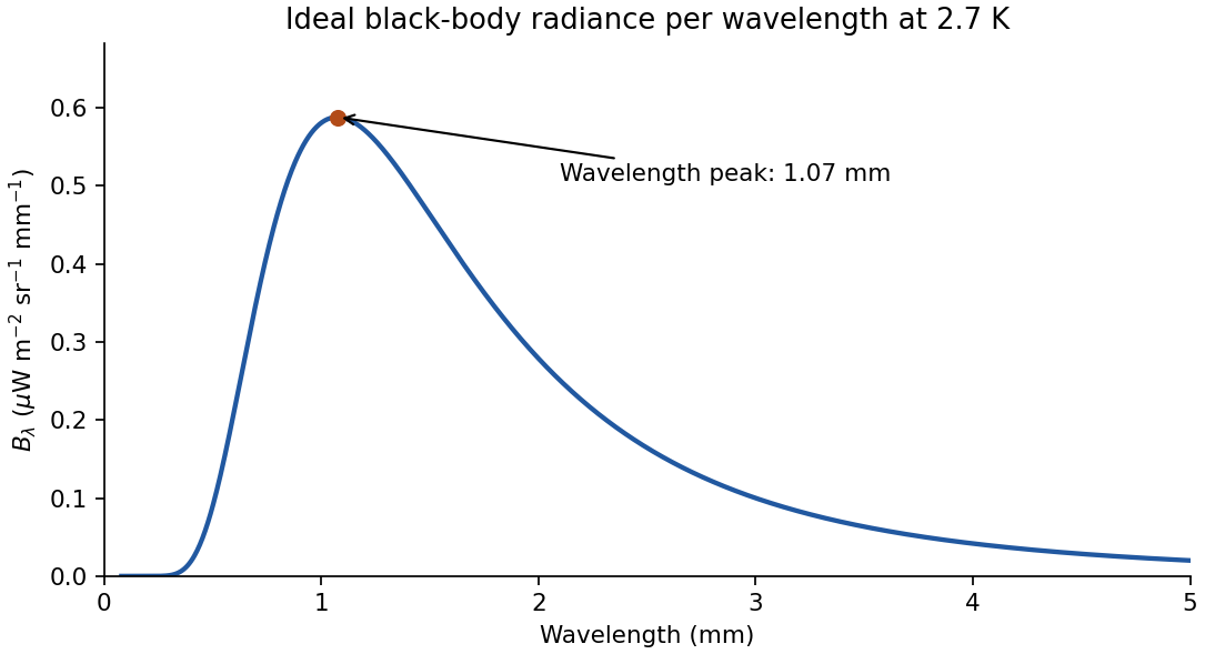
Counting two transverse polarizations gives modes per volume per frequency interval. Thus the spectral energy density is . In an isotropic radiation field, spectral radiance is . Transforming the spectral measure, , givesHere intensity means radiance per wavelength and solid angle; the hemispheric spectral exitance of a black surface is . The extra Jacobian is essential: the wavelength peak is not found by simply converting the frequency peak using .
At short wavelength the exponential suppresses radiation. At long wavelength the Rayleigh-Jeans limit is ; using classical equipartition at every frequency instead would produce the ultraviolet catastrophe. The wavelength maximum solves , with nonzero root , yielding Wien's displacement law. For the specified temperature,Integrating the hemispheric flux gives the Stefan-Boltzmann law, . The plot uses the specified ideal temperature, rather than substituting a later measured value. The physical black-body description of the cosmic microwave background is tested by comparing the sky spectrum with an absolute reference blackbody and separating instrumental and Galactic contributions.[ref]
The Cosmic Microwave Background Spectrum from the Full COBE/FIRAS Data Set by Dale J. Fixsen and others. abstract; FIRAS comparison with a precise blackbody and limits on spectral residuals


For a normalized top-hat wavefunction of width centred at zero, inside the interval and zero outside. Its position distribution has and . With Fourier convention , the momentum amplitude isThe momentum density has long oscillatory tails. Consequently diverges: the ideal discontinuous top hat has infinite r.m.s. momentum spread. Its symmetric momentum density has formal principal-value mean zero, but no finite absolute first moment either. The finite-variance form is therefore not saturated and cannot be evaluated using the width of the central diffraction lobe as .
The first momentum zeros occur at , showing the inverse-width scale. Smoothing the edges sufficiently gives a finite momentum variance and restores the ordinary finite-variance uncertainty comparison; sharper edges require larger high-momentum components. It is the ideal jump, not a violation of the uncertainty principle, that causes the divergence.
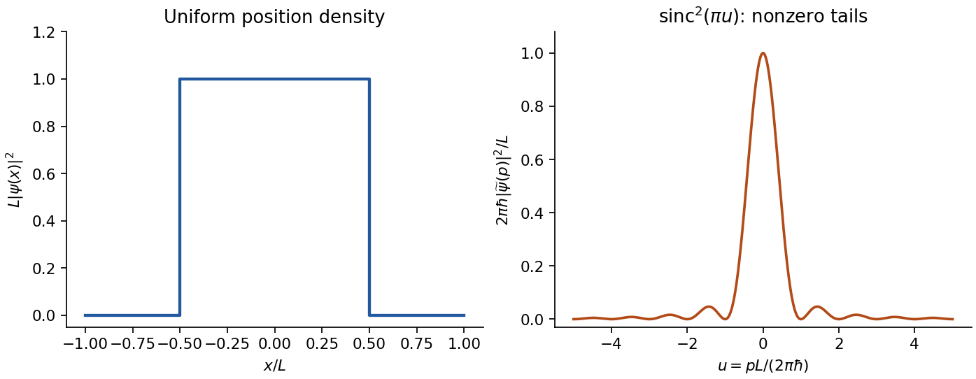
Original top-hat position density and sinc-squared momentum density; the latter has tails giving divergent momentum variance
. Details. 
In a classically forbidden region the local wavevector becomes imaginary. For a slowly varying barrier, the WKB transmission probability has leading exponentialwhere are turning points and is the reduced mass. This is a probability exponent; the wave amplitude has only half that exponent. Near a turning point one uses matching formulas rather than the unmodified local WKB expression.
For alpha decay, an attractive nuclear interior supports a quasibound state behind the repulsive Coulomb barrier of the daughter nucleus. For zero orbital angular momentum, write the exterior potential as , , with nuclear matching radius and outer turning point . The exterior action can be integrated:The decay rate is approximately and the half-life is . Here is the interior assault-frequency scale and is the alpha preformation probability. They are model-dependent; barrier penetration alone does not determine them. Nonzero orbital angular momentum adds a centrifugal barrier.
For , the leading dependence is . Thus a modest increase in decay energy can cause an enormous increase in decay rate, giving the Geiger-Nuttall law relating logarithmic half-life to inverse square-root energy along a suitable isotope sequence. Tunnelling conserves the total energy: the escaping alpha particle does not acquire energy from the barrier.
electron spin is intrinsic angular momentum, independent of an orbital wavefunction's . It has , soA spatial orbital therefore carries a two-component spinor degree of freedom. Noncommuting components do not describe an ordinary vector with simultaneously definite projections; measurements along one axis give only the two allowed values. Even a spherically symmetric orbital retains electron spin.
The associated magnetic moment is with and . A spinor changes sign under a rotation and returns under ; that sign is observable only relative to another coherent amplitude, not as an isolated global phase. A literal classically rotating charged sphere does not account for this fixed half-integer representation, component algebra and spinor rotation law. Classical angular momentum provides useful analogies for torque and precession, but no ordinary classical orientation reproduces the full intrinsic quantum spin structure.
Define and use the independent quoted Gaussian errors , with period and exoplanet transit epoch fixed. The model is linear in despite its sinusoidal time dependence. Minimize . With the normal equations areUsing and , the solution isThe residuals in observation order are . Therefore for degrees of freedom, giving reduced . The upper-tail probability is about : the fit is consistent with the stated errors, although five points do not establish a unique physical explanation.
For known errors the covariance matrix is . Equivalently, profiling out the fitted offset givesThis is the one-parameter uncertainty, not the curvature with incorrectly held fixed. Propagating it through the supplied mass relation, and treating its coefficient and as fixed,The symbol in the exoplanet transit epoch denotes periodic copies of the same exoplanet transit phase, not an uncertainty distribution to propagate. No independent error for the empirical mass coefficient was supplied.
Additional independent observations retain positive weight even with twice the error: each has one quarter of the previous per-observation weight. Their information adds to the existing information matrix, so the formal mass uncertainty decreases for informative additional orbital phases and cannot increase under this fixed-error model. It can remain unchanged in a degenerate phase configuration that supplies no further amplitude information after fitting the offset. The conclusion assumes the same correct model and independent errors, not a new fitted error rescaling or unmodelled systematic effects.
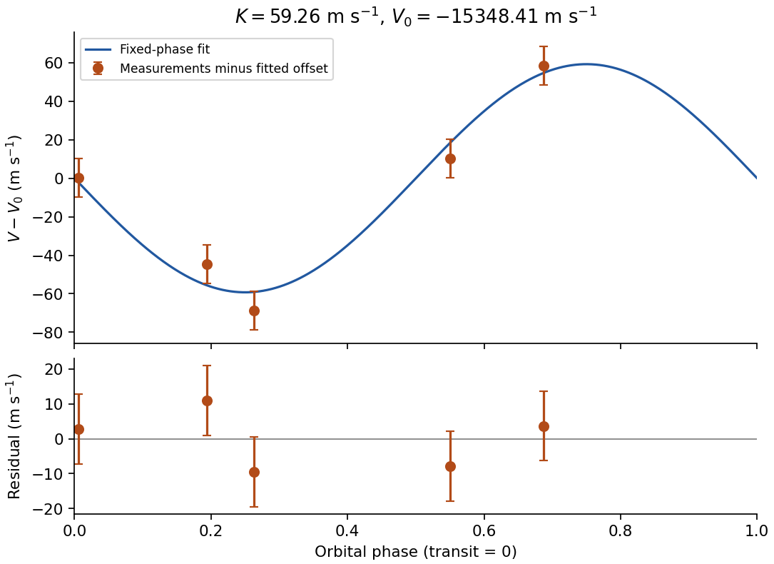
Original plot of the fitted orbital radial-velocity variation and residuals; observed numbers used without reproducing the source table
. Details. 
In an operational-amplifier negative feedback loop, an operational amplifier has large open-loop gain , with . Feeding a fraction back to the inverting input opposes an output increase. For a non-inverting signal input,Its sensitivity to open-loop gain changes is reduced by . Thus resistor ratios can set a reproducible gain despite device variation; feedback also suppresses internal distortion and reduces output impedance. Gain is traded for usable bandwidth, subject to the amplifier's frequency response.
For the non-inverting connection, place between output and inverting input and between that input and ground. Then , giving gain . For an inverting connection, ground the non-inverting input, inject the signal through and return from output to the inverting node. Small differential input and negligible input current then give gain . The near-zero node is a virtual ground, not a physical ground connection.
The feedback must remain stable at the frequencies where loop gain matters. Extra phase lag can turn the intended opposition into oscillation; adequate phase margin, supply headroom, input common-mode range, output-current capability and slew rate are required. Feedback neither prevents clipping nor removes all input noise.[ref]
A lock-in amplifier multiplies the measured signal by a synchronized reference and low-pass filters the product. For and reference , the signal product is . Averaging away the second harmonic gives in this peak-amplitude convention. A second reference gives , soA single quadrature could read zero for a substantial signal from its reference. Two quadratures avoid that blind spot; the phase is undefined at zero amplitude. Instrument RMS calibrations can include a different constant normalization.
The reference shifts the wanted frequency to zero, where a narrow low-pass bandwidth can select it. Uncorrelated broadband noise averages down, whereas a simple amplifier would enlarge signal and noise together. Longer averaging improves narrow-band sensitivity but slows the response to changing amplitude. The signal must remain phase coherent with the reference; frequency mismatch creates a beat instead of a constant output. interference at the same reference frequency survives, so shielding and independent background measurements remain necessary.[ref]
Model SR830 DSP Lock-In Amplifier manual by Stanford Research Systems. printed pp.3-1–3-3, multiplication, dual-phase detection and RMS-versus-peak conventions
Sampling at makes a frequency indistinguishable from , since the extra phase is . For a real sinusoid, reflection to also gives an alias, up to phase. For example, a cosine sampled at has exactly the samples of a cosine. A measured low-frequency feature can therefore originate above the instrument's Nyquist frequency.
To reconstruct an arbitrary baseband signal limited to bandwidth , sample strictly above and use an analogue anti-aliasing filter before the sampler. A practical filter needs a transition band, so merely choosing a nominal rate is insufficient. frequency components already folded together cannot in general be separated by later digital filtering. aliasing from insufficient sampling is distinct from spectral leakage caused by a finite observation window.
Articles by others on the same topic
There are currently no matching articles.