Let the unit normal point from layer 1 to layer 2. The electrostatic electric field boundary condition is , while Gauss's law for the electric displacement field gives . Here denotes absolute permittivity; replace it by if dielectric constants are relative.
In the steady conducting state, charge conservation makes the normal current density the same in both layers:Writing , the steady fields in two leaky dielectric layers areThe signed interfacial free surface charge density is the jump of :The total free-plus-bound sheet charge instead follows from the vacuum form of Gauss's law,The bound contribution is . These are signed quantities for the chosen normal and voltage direction; their magnitudes are obtained by absolute values. They describe the long-time DC state, not the initial capacitive transient. Positive conductivities suffice for the derivation; if both vanish, conductivity alone does not determine the field division, which also depends on the initial free interfacial charge.
Faraday's law for a moving circuit is . The magnetic flux is through a surface bounded by the instantaneous loop, with consistent orientation. For the stationary external field here, the motion supplies the motional electromotive force.
Let be downward penetration of the bottom segment, , and . While , flux grows at rate . Define positive current as the direction whose magnetic force is upward. With negligible self-inductance, andThe resistive magnetic entry of a falling loop givesThe initial acceleration is and the speed approaches if the loop remains partly immersed long enough. Joule heating removes gravitational energy. At the first , both horizontal segments are inside the uniform field: the net flux becomes constant, the net magnetic force vanishes, and this zero-inductance model has thereafter. The subsequent speed increases with acceleration .
For negligible electrical resistance, conservation of total linked flux instead gives in the braking-current convention. Thereforeand the lossless limit of magnetic loop braking yieldsHere energy is stored reversibly in , not dissipated. If , the loop reverses before complete entry and executes the ideal oscillatory motion while straddling the boundary. If , it reaches complete entry on its first descent; thereafter the current is constant, the forces on its two horizontal segments cancel, and it falls with acceleration . The exact grazing case needs care at the ideal discontinuous field boundary. An entry-only sinusoid must not be extrapolated through full immersion.
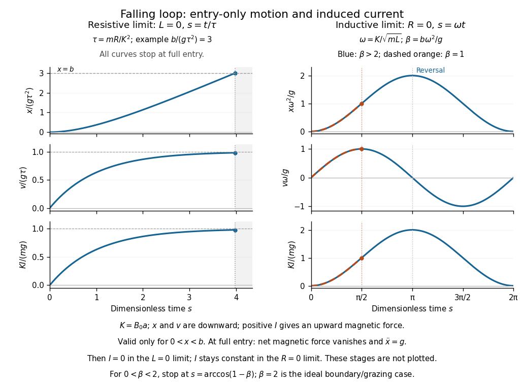
Resistive relaxation and reversible inductive motion during loop entry
. Original dimensionless entry solutions. Curves assume that the loop is long enough for the indicated stage; a fully immersed loop has different subsequent dynamics. Details.
The fundamental mode of an ideal coaxial cable is a transverse electromagnetic mode: the electric field is radial between the conductors, the magnetic field is azimuthal, and energy flows along the cable through the dielectric. There is no cutoff for this mode; higher modes, conductor losses and dielectric dispersion can matter outside the ideal transmission-line regime.
Ignoring edge fields in the parallel-strip geometry, and . Per unit length the charge is and the linked magnetic flux is . Thus the parallel-plate transmission line hasFor a segment , charge conservation, equivalently the appropriate integral of the Ampère-Maxwell equation, gives . Applying Faraday's law around a longitudinal rectangle between the plates gives . These are the lossless telegrapher's equations,Differentiate the second with respect to and use the first, and conversely for :The signal speed is , equal to for a vacuum-filled line. It is the speed of the coupled electromagnetic disturbance, rather than the electron drift velocity. Electrons locally adjust their motion as the field arrives; one electron need not travel the cable's length to transmit a signal. The Poynting vector in the dielectric integrates to power .
The method of images replaces conductors by fictitious charges chosen to reproduce their boundary potentials in the physical domain. The uniqueness theorem for the electrostatic potential then identifies the resulting physical exterior field; the fictitious interior field is not the field inside the conductor.
For a source at , let and . At a point on , the distances and to source and image obey . Hence everywhere on the sphere. This proves the image charge for a grounded conducting sphere construction.
With real charges at , superpose two images of charge at . For the right-hand charge, take positive force away from the centre. Its electrostatic force isPutting , the equal-charge balance around a grounded sphere requiresFor large , the right side is approximately , so . This is an approximate equilibrium, not an exact cancellation at .
To hold the sphere at electric potential , add a central image . The grounded pair already contributes zero potential on its surface. ThereforeAt this is , or approximately if the small grounded residual is neglected as in the preceding approximation. The charge on the sphere is ; fixing its potential is different from independently fixing its net charge.
Articles by others on the same topic
There are currently no matching articles.