Original paper: Public original PDF, physical pages 265–272.
For a reversible isothermal expansion of one mole of an ideal gas, internal energy depends only on temperature, so . The first law of thermodynamics givesThis uses quasistatic expansion against the gas pressure. Specifying only the initial and final volumes and constant temperature would not fix heat for an arbitrary irreversible process: an insulated ideal-gas free expansion has .
Take the wires along , with the first at carrying , and observe at . The Biot-Savart law gives a first-wire field in ; wire is away. ThereforePairing adjacent terms, with ,Thus . Its direction is opposite to the field of the first wire at the observation point. Reversing every electric current reverses this answer.
An empty perfectly conducting rectangular electromagnetic waveguide hasThe lowest transverse electric mode has indices or . A simply connected hollow metallic guide has no transverse electromagnetic mode. With , the two lowest modes are degenerate and their cutoff frequency isPropagation with nonzero axial energy transport requires ; the equality is the lower limiting frequency, with zero axial group velocity. A filling medium would replace by .
Suppose two distinct reversible adiabatic processes intersect at an equilibrium state . Choose an isothermal process that meets the two branches at distinct states and , forming a nonzero-area three-sided thermodynamic cycle. There is no heat exchange on or , so the only net heat comes from the one heat reservoir on . Since around a cycle, .
Choose the direction in which this nonzero cycle delivers positive work. It would then convert heat from a single reservoir entirely into work, violating the Kelvin-Planck statement of the second law. Distinct reversible adiabats cannot intersect. Equivalently, their constant entropy labels cannot differ at one equilibrium state. The argument concerns an ordinary equilibrium family of reversible adiabats, not arbitrary irreversible insulated paths. The usual local uniqueness of an equilibrium adiabat excludes coincident segments described as distinct curves.
The trihydrogen cation is a nonlinear three-nucleus molecule. Removing three translations and three rigid rotations leaves vibrational degrees of freedom. One normal mode is the symmetric in-plane breathing motion: every nucleus moves radially toward or away from the centre. The remaining two normal modes form a degenerate in-plane distortion pair, stretching one direction while compressing another.
For an explicit sketch, let be the equilibrium vertices relative to their centre. Displacements proportional togive the breathing mode and a basis of the degenerate pair. Linear combinations within the latter pair are equally valid. Their actual frequencies require molecular force constants, which are not supplied. An apparent out-of-plane motion of three point nuclei is a translation or infinitesimal rigid rotation, rather than an additional independent vibration.
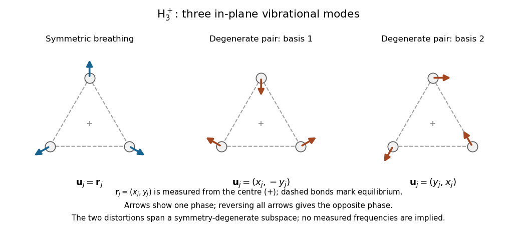
Breathing and degenerate distortion modes of an equilateral molecule
. Original displacement vectors in a simple symmetric bond-spring illustration. The degeneracy is fixed by symmetry; no measured molecular frequencies are asserted. Details.Let the unit normal point from layer 1 to layer 2. The electrostatic electric field boundary condition is , while Gauss's law for the electric displacement field gives . Here denotes absolute permittivity; replace it by if dielectric constants are relative.
In the steady conducting state, charge conservation makes the normal current density the same in both layers:Writing , the steady fields in two leaky dielectric layers areThe signed interfacial free surface charge density is the jump of :The total free-plus-bound sheet charge instead follows from the vacuum form of Gauss's law,The bound contribution is . These are signed quantities for the chosen normal and voltage direction; their magnitudes are obtained by absolute values. They describe the long-time DC state, not the initial capacitive transient. Positive conductivities suffice for the derivation; if both vanish, conductivity alone does not determine the field division, which also depends on the initial free interfacial charge.
Faraday's law for a moving circuit is . The magnetic flux is through a surface bounded by the instantaneous loop, with consistent orientation. For the stationary external field here, the motion supplies the motional electromotive force.
Let be downward penetration of the bottom segment, , and . While , flux grows at rate . Define positive current as the direction whose magnetic force is upward. With negligible self-inductance, andThe resistive magnetic entry of a falling loop givesThe initial acceleration is and the speed approaches if the loop remains partly immersed long enough. Joule heating removes gravitational energy. At the first , both horizontal segments are inside the uniform field: the net flux becomes constant, the net magnetic force vanishes, and this zero-inductance model has thereafter. The subsequent speed increases with acceleration .
For negligible electrical resistance, conservation of total linked flux instead gives in the braking-current convention. Thereforeand the lossless limit of magnetic loop braking yieldsHere energy is stored reversibly in , not dissipated. If , the loop reverses before complete entry and executes the ideal oscillatory motion while straddling the boundary. If , it reaches complete entry on its first descent; thereafter the current is constant, the forces on its two horizontal segments cancel, and it falls with acceleration . The exact grazing case needs care at the ideal discontinuous field boundary. An entry-only sinusoid must not be extrapolated through full immersion.
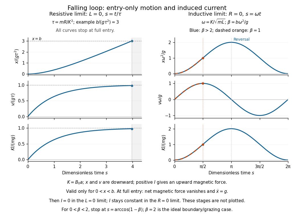
Resistive relaxation and reversible inductive motion during loop entry
. Original dimensionless entry solutions. Curves assume that the loop is long enough for the indicated stage; a fully immersed loop has different subsequent dynamics. Details.The fundamental mode of an ideal coaxial cable is a transverse electromagnetic mode: the electric field is radial between the conductors, the magnetic field is azimuthal, and energy flows along the cable through the dielectric. There is no cutoff for this mode; higher modes, conductor losses and dielectric dispersion can matter outside the ideal transmission-line regime.
Ignoring edge fields in the parallel-strip geometry, and . Per unit length the charge is and the linked magnetic flux is . Thus the parallel-plate transmission line hasFor a segment , charge conservation, equivalently the appropriate integral of the Ampère-Maxwell equation, gives . Applying Faraday's law around a longitudinal rectangle between the plates gives . These are the lossless telegrapher's equations,Differentiate the second with respect to and use the first, and conversely for :The signal speed is , equal to for a vacuum-filled line. It is the speed of the coupled electromagnetic disturbance, rather than the electron drift velocity. Electrons locally adjust their motion as the field arrives; one electron need not travel the cable's length to transmit a signal. The Poynting vector in the dielectric integrates to power .
The method of images replaces conductors by fictitious charges chosen to reproduce their boundary potentials in the physical domain. The uniqueness theorem for the electrostatic potential then identifies the resulting physical exterior field; the fictitious interior field is not the field inside the conductor.
For a source at , let and . At a point on , the distances and to source and image obey . Hence everywhere on the sphere. This proves the image charge for a grounded conducting sphere construction.
With real charges at , superpose two images of charge at . For the right-hand charge, take positive force away from the centre. Its electrostatic force isPutting , the equal-charge balance around a grounded sphere requiresFor large , the right side is approximately , so . This is an approximate equilibrium, not an exact cancellation at .
To hold the sphere at electric potential , add a central image . The grounded pair already contributes zero potential on its surface. ThereforeAt this is , or approximately if the small grounded residual is neglected as in the preceding approximation. The charge on the sphere is ; fixing its potential is different from independently fixing its net charge.
For steady inviscid incompressible flow subject to a conservative body force, Bernoulli's theorem states that is constant along a streamline. The same constant applies across streamlines only with an additional condition, such as an irrotational connected flow with the same upstream head.
Neglect gravity and let the film's free-surface pressure be atmospheric. Its radial speed is then in the ideal model. Conservation of mass equates the incoming flux to , soThe latter value already warns that the thin-film approximation is poor near impact; the radial expression is most useful beyond that region. The incoming vertical momentum flux gives downward force when the outgoing flow is horizontal.
In the stipulated stagnant-rear-layer idealization, the excess rear pressure is the stagnation value . Its upward force is . Thus, with downward positive and ignoring the water's weight,For a large plate, the radial-film volume is approximatelyIts weight therefore changes the model toCancellation occurs nearThe printed claim of negligible force for every radius above this scale does not follow from this model. Near the cancellation radius the force is small; for substantially larger radii the quadratic upward-pressure term dominates. The original PDF, not just its transcription, uses that inequality and wording. Moreover, the rear layer's mass and detailed gravity-dependent pressure field are unspecified. The calculation establishes a cancellation scale under the elementary stated pressure approximation, rather than a general large-radius zero-force theorem. A full free-surface flow model would be needed to extend it consistently.
For a Lagrangian , the Euler-Lagrange equation is for each unconstrained generalized coordinate. For example, gives for a spring oscillator.
For a uniform solid sphere, slicing into disks normal to the rotation axis givesUse total dumb-bell mass and . Since both centres lie on its spin axis, its moment of inertia about that axis is . If measures displacement from the bottom of the track, rolling without slipping imposes spin speed . The rolling inside a fixed circular cylinder therefore hasThe equation of motion and its small-amplitude limit areWith and the given lengths, . If the centre rises by height , conservation of energy at the bottom givesThe speed expression uses exact height-energy conversion within the ideal rolling constraint; only the period formula uses the small-angle approximation.
Let be the polar second moment of area. A twist gradient gives shear strain and shear stress . Integrating its moment over a cross section yieldsThe difference in torque on an element is , while its angular inertia is . Hence the torsional wave equation in a circular shaft isFor uniform rotation at , transmitted power is , so the given values give . The elastic strain energy and rotational kinetic energy areThe torsional transit time is . If the requested maximum rates mean stored-energy-over-transit-time estimates, they areThese estimates require a physical qualification. They are not separate upper bounds on transmitted mechanical power. The exact local energy flux of a torsional wave is the stress-work rateFor the steadily rotating twisted shaft its magnitude is , even though this exceeds . Writing local energy densities and gives . A single travelling torsional wave has equal strain and kinetic energies; the steady shaft can instead be represented by oppositely travelling components whose powers largely cancel. Its stored strain pattern is not a fuel consumed once per transit. This distinguishes an energy-content estimate from the actual stress-mediated transport.
In plane polar coordinates the radial component of Newton's second law is . A central force has zero torque, so angular momentum is constant. ThereforeFor a nonzero-angular-momentum circular orbit at , . The curvature there isThus a stable circular orbit, and nearby bound orbits, require , with excluded. For , confines the particle at large radius; for , permits bound energies between the effective-potential minimum and zero. At there is no isolated stable minimum.
The angular frequency is , and radial perturbations have frequency . A rational ratio closes the linearized near-circular trajectory. It does not prove finite-amplitude closure. Bertrand's theorem supplies the stronger conclusion: every bound orbit is closed only for and among these smooth attractive power-law potentials. Particular circular or resonant orbits must not be confused with that all-orbit statement.
For , the slowly rotating elliptical orientation has angular speedThis is retrograde for in the near-circular approximation. Consecutive radial maxima are separated by approximately in azimuth; the ellipse's axis is defined modulo , which accounts for the factor of two relative to a Kepler-style apsidal convention.
Source for this section: Physical PDF pages 271–272, printed pages 7–8 of Physics B (2A), 2 June 2010.
A normal mode has all displacement coordinates proportional to a common time dependence, with fixed relative amplitudes. For a nonzero frequency the time dependence is sinusoidal. A zero-frequency mode is a free displacement or uniform drift rather than an oscillation.
Use the printed mass ordering . Displacements are measured from the unstretched equilibrium positions, givingEquivalently,This is the generalized eigenvalue problem for normal modes of three masses connected by two equal springs. Substitute to obtain . Reflection symmetry gives an antisymmetric vector and symmetric vectors . The former has . For a symmetric vector, the end and centre equations give and . Their solutions are , , or , . HenceThese are all three eigenmodes. The last two keep the centre of mass fixed and are orthogonal in the mass-weighted inner product. The general zero-mode contribution is , accounting for both a centre-of-mass shift and a conserved total momentum. There are no fixed end springs in this system.
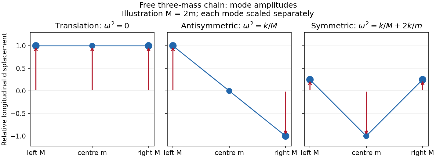
Free-chain mode shapes
. Details. The original amplitude profiles illustrate ; the symmetric internal shape is rescaled for display. The formula above gives every positive mass ratio.
Two further physical examples are standing-wave modes of a string fixed at both ends, with spatial shapes and frequencies , and electrical normal modes of two coupled LC circuits, in which the capacitor charges oscillate at fixed relative amplitudes. Independent normal mode coordinates simplify both systems in the same way as the spring-chain eigenvectors.
A Fourier series separates a periodic physical signal into harmonics. For example, a periodic voltage applied to a linear circuit can be treated one frequency at a time; the harmonic responses then superpose to give the output waveform.
Write for the pulse width and for its duty cycle, with . The waveform is a train of positive rectangular pulses centred on , each with area one. It is even about , so every sine coefficient vanishes. Cosine orthogonality givesand, for ,This is the Fourier series of a periodic rectangular pulse:The actual constant term in the series is , not . As usual for a jump discontinuity, the series converges to the average of the one-sided values at each pulse edge, namely , irrespective of the value assigned at that isolated endpoint. Elsewhere it converges to the rectangular waveform.
Counting the constant as the first term, the first three terms areso their sum isIf “first three” instead means the first three nonconstant harmonics, add ; the original plot shows that alternative partial sum as well. The three-term approximation rounds the narrow peaks and ripples between them; many harmonics are needed to represent a sharp pulse.
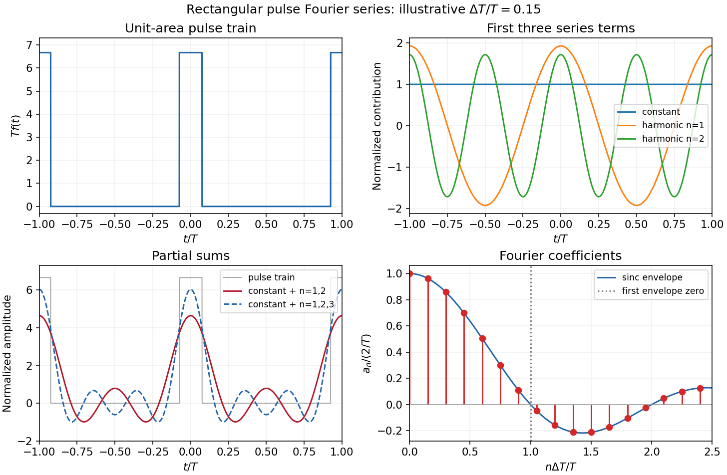
The original sketches use the illustrative duty cycle and cover . The coefficient panel also displays the first spectral zero.
For , expand the sinc function:Thus the low-index coefficients, including , have nearly equal values, although their constant-series contribution still has the factor . The first sinc zero occurs at , or . If this is not an integer, the closest integer coefficient is near zero rather than exactly zero: writing gives . This pulse-width scale of Fourier coefficients means that a narrower pulse requires significant harmonics extending to proportionally larger indices, the reciprocal time-width/frequency-width relation.
Linearity means that the differential operator obeys . Therefore any linear combination of homogeneous solutions is again a solution; associated initial or boundary data must be combined by the same rule.
With characteristic coordinates and , the equation becomes . Integrating in these coordinates givesThe two profiles propagate without changing shape at speeds and . Equivalently write . At , the data imply and . Hence is constant; its two contributions cancel in , givingThe slope formula holds classically wherever the two derivatives exist, and as a weak derivative otherwise. Since the string tension is , here must be mass per unit length. These are two-sided string data with zero slope. The stipulated boundary data specify incoming as well as outgoing waves; this is not a pulse generated on an everywhere initially resting infinite string. For example, at a positive observation point its incoming signal can begin before the motion at begins.
For explicit profiles put , andThen and . At ordinary points, for and zero for . Because itself vanishes at both support edges, this first weak derivative has no delta-function term, although it has jumps.
At , the displacement isFor non-front times its slope isThis is displacement cancellation without slope cancellation in crossing pulses: displacement cancels throughout the overlap , but slope generally does not. Cancellation at one spatial position for an interval of time does not imply cancellation of the spatial derivative there. At , the classical slope is not defined; the adjacent pieces specify its one-sided limits.
At the two windows meet without an open overlap. Their displacements combine intowith slopeAt the classical slope is undefined. At the exceptional meeting time , oddness of gives for every , so the spatial derivative is exactly zero there. Its one-sided time limits at are and ; these do not determine its value at the meeting point.
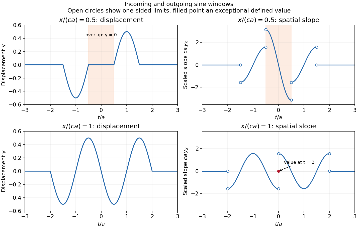


The original graphs distinguish continuous displacements, open-ended one-sided slope traces, and the zero slope at the isolated meeting point. The sharp temporal window is not differentiable at its endpoints, so the overall solution is piecewise classical and globally weak. In particular the literal boundary slope at is not a classical derivative: the even spatial profile has a cusp there. The zero-slope boundary prescription is satisfied at regular times and in its almost-everywhere trace sense; it cannot be read as a globally smooth classical condition for this nonsmooth .
Stokes theorem converts circulation around an oriented boundary into curl flux through a spanning surface. For a sufficiently smooth vector field on an oriented piecewise smooth surface ,The boundary orientation follows the right-hand rule relative to . The field must be smooth on the surface, not merely on its boundary; a singularity crossing the surface cannot be ignored. For a fixed loop, applying the theorem to Faraday's differential law gives the integral flux law of induction.
The planar form is Green theorem. For a region with positively oriented boundary and sufficiently smooth ,The outer boundary is counterclockwise and any holes have clockwise boundaries. For instance makes the area of equal to half the line integral of ; the unit circle gives area .
A closely related use of “Green's theorems” in field theory is Green's identities, obtained by applying the divergence theorem to :and, after subtracting the expression with exchanged,These relate interior sources to boundary data in electrostatics and other boundary-value problems. For example, a harmonic potential difference vanishing on a Dirichlet boundary condition has zero integral of its squared gradient by the first identity, establishing uniqueness. Both the planar circulation theorem and the field identities are included here to make the convention clear.
Separation of variables replaces a compatible partial differential equation by ordinary differential eigenvalue equations. For example, with a thermally diffusive rod, , try . Wherever division is valid,The two sides depend on independent variables, so each must be constant. Homogeneous end temperatures give and . The general initial-temperature profile is represented by superposing these separated modes:Each spatial mode decays at its own rate. For a fixed-end wave equation the same spatial eigenfunctions instead have oscillatory time factors , with coefficients fixed by initial displacement and velocity. Similar constructions separate Laplace's equation in suitable coordinate systems.
A single product is usually only one mode, not the most general solution. Linear superposition and completeness of the spatial eigenfunctions are what extend the method to general allowed data. Nonhomogeneous boundary values can first be removed by a known stationary or particular solution. Separation is effective when the geometry, coefficients and boundary conditions admit a common separated eigenproblem; an arbitrary nonlinear equation or inseparable geometry need not do so. Self-adjoint Sturm-Liouville problems explain the weighted orthogonality and completeness in many physical applications.
Convolution describes the response of a linear time-invariant system to an arbitrary input. If is its impulse response and its input,This is a weighted sum of responses to shifted impulses. For integrable functions the operation is commutative and associative. A causal system has for , restricting the integral to past inputs. With the Fourier convention , the convolution theorem gives .
For example, an RC low-pass frequency response has and , where is the Heaviside step function. Fast input variations are smoothed. The same mathematics describes optical blurring by a point spread function and many other linear response measurements.
Deconvolution tries to recover from measured and known . In noise-free data one formally sets where . Zeros of lose corresponding information; small values amplify measurement noise. If the measured spectrum is , the direct estimate has error , which can be very large at frequencies strongly suppressed by the instrument. An inverse is therefore not automatically unique or stable.
One regularized spectral deconvolution reconstruction isThis minimizes at each frequency and limits noise amplification, at the cost of bias and lost resolution. Choosing the regularization requires assumptions about noise and the desired signal; deconvolution cannot restore components that the data do not determine without such additional information.
Orthogonality means zero inner product, not merely that two objects look different. For complex vectors, ; for functions a common choice is with positive weight . An orthonormal set has .
For an orthogonal set, the component of along has coefficientA complete orthonormal set gives in the appropriate norm and Parseval's identity . Without completeness there can be a nonzero residual orthogonal to the entire chosen set. Orthogonal nonzero vectors are linearly independent, but independence alone does not imply orthogonality.
Fourier coefficients are projections becauseLikewise, for a self-adjoint operator, gives , so distinct eigenvalues have orthogonal eigenvectors. Degeneracy does not itself force a chosen pair to be orthogonal, but an orthonormal basis can be selected within each eigenspace. The differential version uses the correct Sturm-Liouville weight and boundary conditions.
For mechanical normal modes with unequal masses the relevant inner product is . This makes the modes in D14 orthogonal even when an ordinary unweighted dot product does not. Expanding in such coordinates diagonalizes the kinetic and potential quadratic forms, explaining why modal motions evolve independently and their energies add.
Articles by others on the same topic
There are currently no matching articles.