Past exam of the short options paper shared by Prelims and Parts A and B of the physics course of the University of Oxford / 2012 / S25 / 2

Hydrostatic equilibrium balances the vertical pressure gradient against weight, $dP/dz=-\rho g$. For a dry ideal gas parcel displaced slowly enough to maintain pressure balance but rapidly enough to exchange negligible heat, the first law givesCombining the two equations yields the dry adiabatic lapse rateusing $c_p\simeq 1004\mathrm{J}\mathrm{k}{\mathrm{g}}^{-1}{\mathrm{K}}^{-1}$. Here temperature in the thermodynamic differential is absolute, $g$ and $c_p$ are treated as constant, composition is fixed, and condensation is excluded. Hydrostatic balance alone does not force the atmosphere to be adiabatic; the parcel assumption supplies the extra relation.

Water condensation releases latent heat, reducing the cooling of a rising saturated parcel and giving a smaller moist adiabatic lapse rate. Radiation, mixing, large-scale motion and incomplete convective adjustment also shape the environmental lapse rate. Thus an observed $6$--$7\mathrm{K}\mathrm{k}{\mathrm{m}}^{-1}$ need not equal the dry parcel value and is broadly consistent with a moist, radiatively influenced atmosphere.

Write $s=T_s-273.15\mathrm{K}$ as the numerical sea-level Celsius temperature in degrees Celsius, and use the same degree increments for $\Gamma z$. The model's top temperature is $T_C=s-\Gamma z$. For positive $\alpha$ its intended cold-ice branch has $T_C<0$, so the positive melt-loss magnitude and snow gain areThe model is singular at $z=s/\Gamma$ and is not a physical melting law across that boundary. On the relevant interval $s/\Gamma <z<1/\beta$, $L$ decreases hyperbolically and $A$ decreases linearly. Assume a fixed area and positive ice density, so increasing mass increases $z$: stability has the same sign as $F^{\prime }(z)$.

The equilibrium equation iswith rootsTwo distinct physical equilibria, one stable, exist providedThis combines a positive allowed interval with a strictly positive discriminant. At the larger root $F^{\prime }<0$ and small perturbations restore the ice cap; the smaller root has $F^{\prime }>0$ and is unstable. Sincea restoring local response requiresThis is the lower height bound from the stability derivative; the stable equilibrium itself is $z_{+}$. The minimum initial height for persistence, a different notion of threshold, is the unstable separator $z_{-}$: initial heights above it approach $z_{+}$, while lower heights lose ice and leave the model's cold branch. At equality in the discriminant condition the two equilibria merge, giving a marginal fold rather than a strictly stable ice cap.

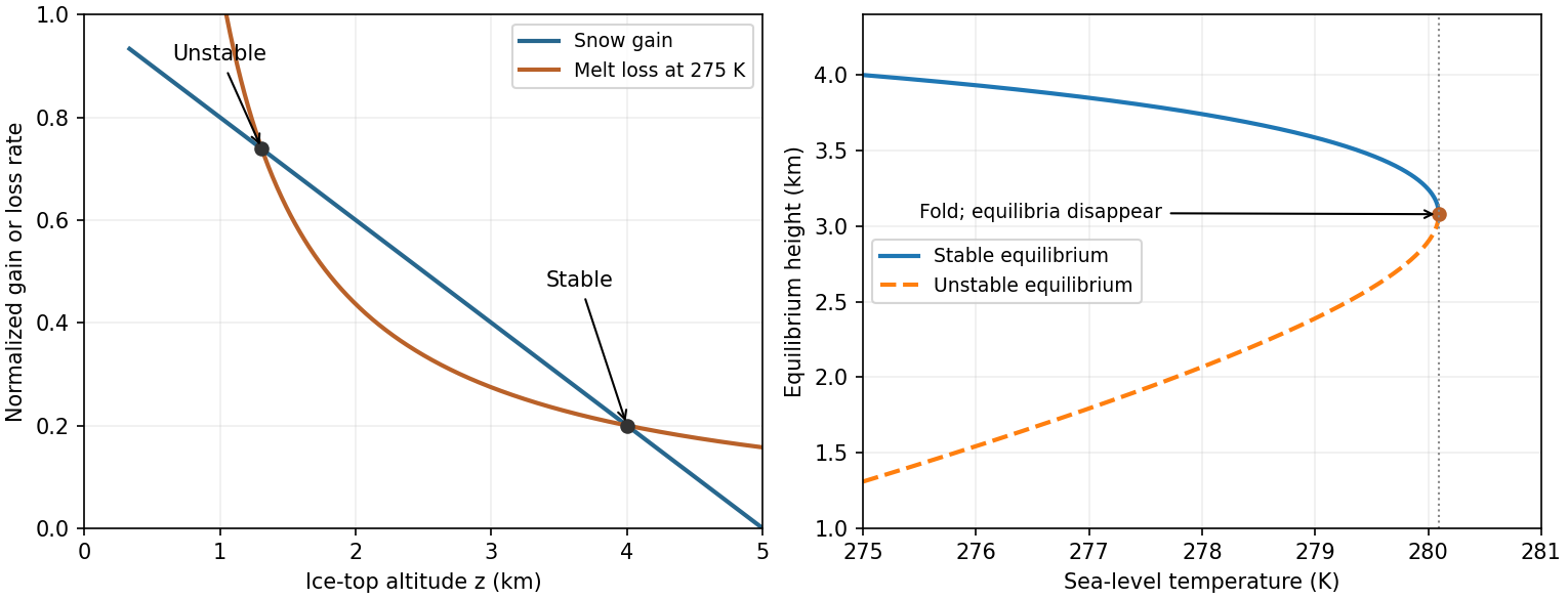
At $z=4\mathrm{km}$, the snow gain is $1-0.2(4)=0.2$ and the model's top Celsius temperature is $275-273.15-6(4)=-22.15^{\circ }\mathrm{C}$. Equilibrium givesin the normalized rate convention. Using $273\mathrm{K}$ for the Celsius zero instead would give $4.4^{\circ }\mathrm{C}$. The local slope is $-0.2+4.43(6)/(22.15{)}^2\simeq -0.1458\mathrm{k}{\mathrm{m}}^{-1}<0$, as required. Initially $z_{-}=1.3083\mathrm{km}$ and $z_{\mathrm{slope}}\simeq 2.230\mathrm{km}$, while $z_{+}=4\mathrm{km}$.

As $T_s$ slowly rises, melt loss increases at fixed $z$, the stable high branch moves downward and the unstable branch upward. They merge atBeyond the fold the model has no steady cold ice cap: its net balance is negative throughout the physical interval and ice shrinks until the assumed law ceases to apply. Quasistatic tracking presumes adjustment is fast compared with the imposed warming, an assumption that deteriorates near the fold as the restoring slope tends to zero. This singular idealized law is not a quantitative real-world melting forecast.