For this concave recruitment map, the extinction state is invariant because . Near extinction, with multiplier above one, so small positive populations initially grow. The strict concavity means marginal recruitment decreases as population increases. More precisely, for ,since . Thus per-capita recruitment decreases and the graph bends downwards from an initial slope greater than that of the identity line.
A positive fixed point, if present, is the unique positive intersection with : the strictly decreasing ratio can cross one at most once. The sketch shows the usual saturating example , which crosses at .
The three assumptions alone do not guarantee this crossing. For example satisfies all three and remains strictly above for every . An extra large-population restriction, such as somewhere, supplies existence. Keeping this distinction avoids inventing a carrying capacity that is not implied by the printed hypotheses.
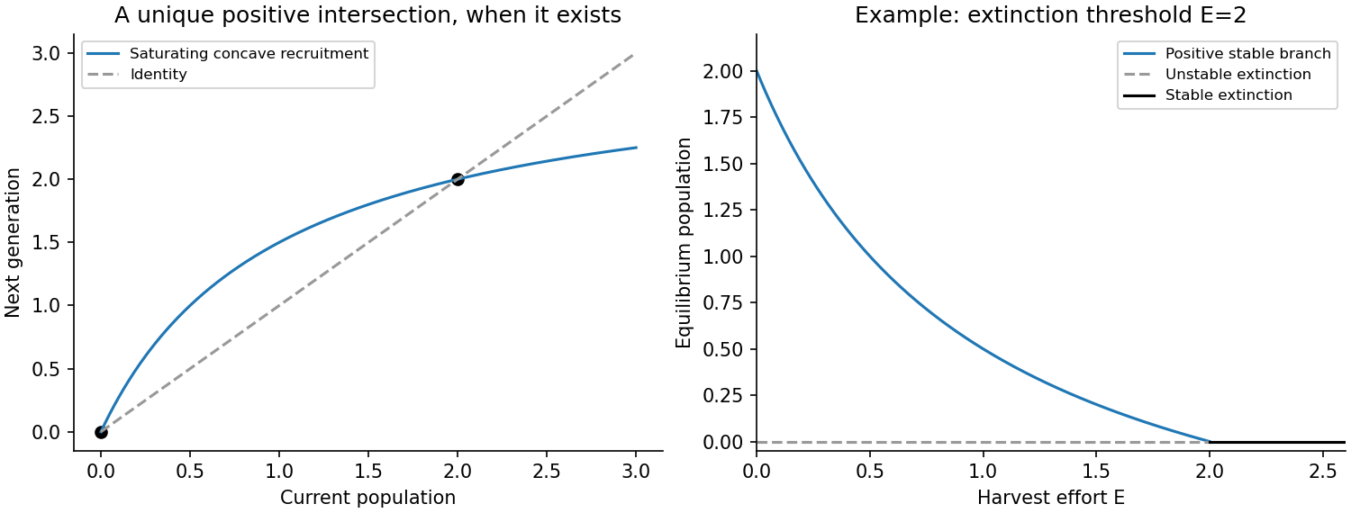
Concave recruitment and the identity line, with loss of the positive equilibrium under harvesting
. Details. 
Let be a fixed point and put . Taylor expansion gives , so the linear perturbation is . Thereforeis the condition for linear asymptotic stability. A multiplier in gives monotone decay; one in gives alternating decay. If its magnitude exceeds one, perturbations grow. Magnitude one is nonhyperbolic and needs nonlinear analysis.
Strict concavity and already give . Thus the remaining stability requirement is . If is additionally nonnegative on the entire half-line, strict concavity prevents its derivative becoming negative there, since it would then force eventually negative. Under that stronger global population-map assumption the positive fixed point is automatically stable. The printed local slope and concavity information, without that global nonnegativity requirement, does not by itself rule out a flip instability.
With constant-effort harvesting, the constant-effort model isThe extinction multiplier becomes , so extinction is linearly stable when . At its multiplier crosses . Values large enough to make the next population negative lie outside the physical validity of this untruncated harvest model.
Any positive fixed point solves . Since that ratio is strictly decreasing, there is at most one such point, and it decreases with effort. Differentiating the fixed-point equation yieldsIf the unharvested positive branch exists, it continues for and approaches zero as . This follows because its required ratio lies between and ; its intersection lies between zero and the unharvested fixed point. There is no positive fixed point for .
The positive-state multiplier is by concavity. It is stable precisely whenCrossing can change stability through a flip, but the direction of change is not fixed by the three assumptions: has no prescribed sign. In the illustrated saturating example, increasing effort eventually removes the positive branch at extinction. The finite upper stability bound for the algebraic extinction map should not be interpreted as a physically meaningful recovery of a population at unrealistically large harvest effort.
A steady population is a root . To linearize one needs differentiable near that root, an extra local regularity assumption beyond the source's continuity. Setting gives , hence at linear order.
Thus gives linear asymptotic stability and gives instability. If , linearization is inconclusive. In a one-dimensional phase line, the more general nonlinear test is whether the vector field points towards the root from both sides. At the physical boundary , only the right-hand side matters. Continuity alone does not guarantee uniqueness of trajectories, so a standard well-defined flow also presumes a local uniqueness condition, such as local Lipschitz continuity.
The four nonnegative equilibria are . Since all factors are positive below , the sign of on consecutive intervals isThe phase line therefore points away from zero, towards , away from , and towards . Equivalently , and at each simple positive root , . Their signs alternate negative, positive, negative.
Hence extinction and are unstable, while and are asymptotically stable. Initial positive populations below tend to ; those above tend to ; an initial population exactly at remains there. This is bistability with a threshold separating the two basins.
Put . The harvested vector field is . Define the extinction threshold , and let be the positive local maximum of , with . Writing , givesPositive equilibria are intersections of with the horizontal line . A lower stable branch in exists exactly for . A pair in exists exactly for : its smaller member has and is unstable; its larger member has and is stable. At a positive root the linear eigenvalue is , which proves these claims. Extinction has eigenvalue , becoming stable for .
The harvested bistable population thresholds determine the behaviour. If , the upper stable population and its unstable separator first disappear in a saddle-node bifurcation. Populations then tend to the remaining lower stable state until that branch reaches extinction at ; beyond it extinction attracts every positive initial state. If , the lower stable branch reaches extinction first. For , extinction and the upper positive state are both stable, separated by the middle unstable root. Increasing effort through then destroys the remaining positive attractor, causing a sudden collapse to extinction. If , both events occur at the same effort at different populations.
At , near zero the leading term is , so extinction attracts from the physical right side algebraically, despite its zero linear eigenvalue. At , the double positive root is semistable: locally , attracting from above and repelling from below. These critical cases matter for exact initial data. The figure shows examples of both strict threshold orderings.
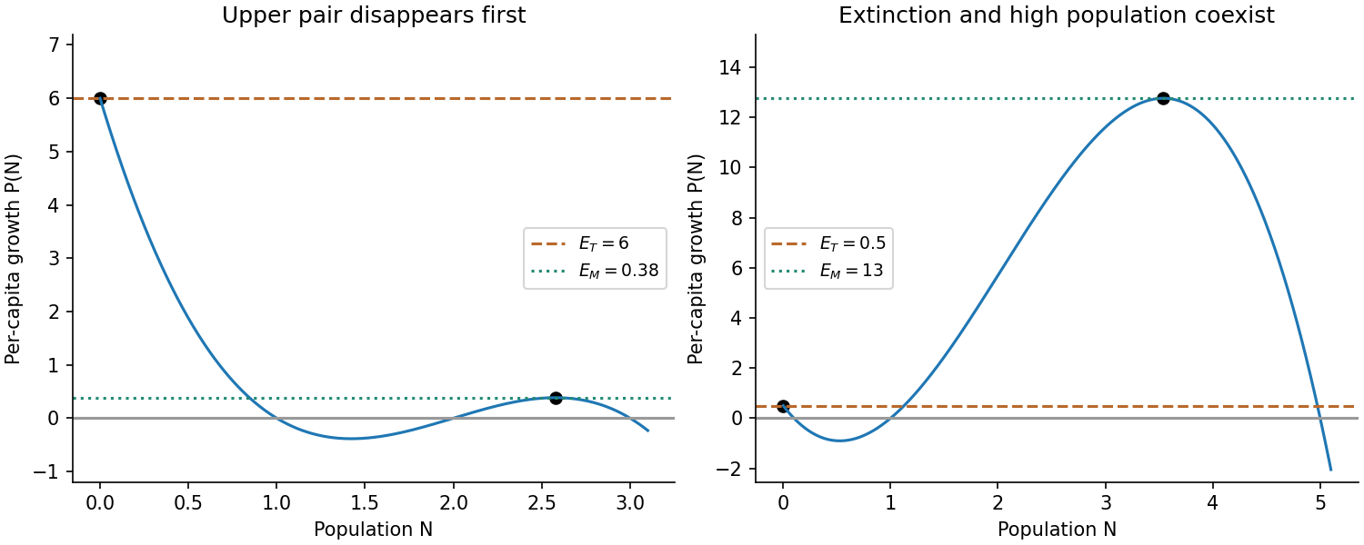
Two possible orderings of the extinction and saddle-node harvesting thresholds
. Details. 
Articles by others on the same topic
There are currently no matching articles.