Functional programming, design and analysis of algorithms (A10097W1)

Solution

Again use structural induction on the finite list. At [], both the right fold and the left fold return e. For x:xs, use reverse (x:xs) = reverse xs ++ [x], part (a), and the definition of flip:

foldl (flip f) e (reverse (x:xs))
= foldl (flip f) e (reverse xs ++ [x])
= foldl (flip f) (foldl (flip f) e (reverse xs)) [x]
= flip f (foldl (flip f) e (reverse xs)) x
= f x (foldl (flip f) e (reverse xs))
= f x (foldr f e xs)
= foldr f e (x:xs)

The penultimate equality uses the induction hypothesis. Thus foldr f e xs = foldl (flip f) e (reverse xs). Finiteness matters: reversing an infinite list does not produce its first element, whereas some right folds do.

c

Solution

Use the right fold definition xs ++ ys = foldr (:) ys xs, the right-identity law xs ++ [] = xs, and the finite-list involution law reverse (reverse xs) = xs. The last two laws are the additional results used here. Part (b) now gives

xs ++ ys
= foldr (:) ys xs
= foldl (flip (:)) ys (reverse xs)

Set ys = [] to obtain xs = foldl (flip (:)) [] (reverse xs). Substitute reverse xs for xs and simplify the double reversal:

reverse xs
= foldl (flip (:)) [] (reverse (reverse xs))
= foldl (flip (:)) [] xs

The derived Haskell definition is therefore

reverse :: [a] -> [a]
reverse = foldl (flip (:)) []

Each step prepends the next element to the accumulator. This is a left fold derivation from list concatenation, rather than merely a proposed implementation.

2

a

Solution

A tree fold first folds every child rose tree, then supplies the resulting list and the current label to the combining function:

foldRTree :: (a -> [b] -> b) -> RTree a -> b
foldRTree f (Node x children) =
  f x (map (foldRTree f) children)

The label type a and result type b are independent, so the polymorphic type needs no class constraint. With f x ys = x + sum ys, every label is counted exactly once; the illustrated labels sum to 28.

The printed source gives the signature exampleRTree but binds exampleRTRee, with different capitalization. They are different Haskell names; the demonstration requires using one spelling consistently. This typo does not affect the tree fold definition.

b

Solution

Compute either the common depth of the leaves of a rooted tree, or failure when the depths differ. A tree fold can return a Maybe Integer: Just h means that the rose tree is a perfect rose tree with all leaves at depth

h

relative to its root; Nothing means it is not perfect.

perfect :: RTree a -> Bool
perfect t =
  case foldRTree step t of
    Nothing -> False
    Just _  -> True
  where
    step :: a -> [Maybe Integer] -> Maybe Integer
    step _ [] = Just 0
    step _ (Nothing : _) = Nothing
    step _ (Just h : hs)
      | all (== Just h) hs = Just (h + 1)
      | otherwise        = Nothing

A leaf has depth zero. An internal vertex has equally deep leaves exactly when every child rose tree is perfect and their returned depths agree; adding one accounts for the edge to each child. This proves the stated meaning of the result by structural induction. In particular, unary branching is allowed, and a single leaf is perfect. perfect returns precisely the required Boolean. Its time complexity is linear in the number of vertices, assuming unit-cost depth arithmetic; labels are never compared or evaluated.

c

Solution

Use concat [] = [], concat (ys:yss) = ys ++ concat yss, the corresponding equations for map, associativity of list concatenation, and (r:ys) ++ zs = r:(ys ++ zs). For an empty forest,

flatten2 [] xs
= concat (map flatten []) ++ xs
= [] ++ xs
= xs

For a nonempty forest, write its first rose tree as Node r children:

flatten2 (Node r children : trees) xs
= (flatten (Node r children) ++ concat (map flatten trees)) ++ xs
= (r : concat (map flatten children))
    ++ (concat (map flatten trees) ++ xs)
= r : (concat (map flatten children) ++ flatten2 trees xs)
= r : flatten2 children (flatten2 trees xs)

Thus the recursive Haskell definition is

flatten2 :: [RTree a] -> [a] -> [a]
flatten2 [] xs = xs
flatten2 (Node r children : trees) xs =
  r : flatten2 children (flatten2 trees xs)

The nested call supplies the continuation of the preorder traversal as a suffix. Each label is emitted once, without repeated list concatenation of an already flattened subtree. For a finite forest, constructing its entire contribution takes linear time in its number of vertices, without traversing the supplied suffix xs.

d

Solution

Measure the work of producing the entire output list, with constant-cost labels. Count height in levels, so a leaf has height one and

h = 0

. A perfect ternary tree with

h + 1

levels has

N_{h} = 1 + 3 + \dots + 3^{h} = \frac{3 ^{h + 1} - 1}{2}

vertices. This is the finite geometric series formula, used without a new proof.

The three recursive calls cost

3 T (h - 1)

. Ordinary concat = foldr (++) [] copies each immediate child result once, and each result has

N_{h - 1}

elements. Consequently the nonrecursive work is

Θ (3 N_{h - 1} + 1) = Θ (3^{h})

, giving

T (0) = Θ (1), T (h) = 3 T (h - 1) + Θ (3^{h}) (h \geq 1) .

Unroll this recurrence relation. At level

j

, the cost is

3^{j} Θ (3^{h - j}) = Θ (3^{h})

, and there are

h

internal levels, followed by

3^{h}

leaves. Therefore

T (flatten) (h) = Θ ((h + 1) 3^{h}) .

(3)

For

h \geq 1

this is conventionally written

Θ (h 3^{h})

; in terms of total size it is

Θ (N_{h} lo g N_{h})

. The extra height factor comes from copying labels at successive ancestors, even under lazy evaluation when the whole output is demanded. Merely producing its first constructor is a different cost question. If height instead counts edges, the source's height

h + 1

means

h + 2

levels; shifting the index by one leaves the boxed asymptotic bound unchanged. Part (c)'s suffix-passing implementation avoids this repeated copying.

3

a

Solution

Only the first constructor needs to be inspected:

headZig :: Zig a b -> a
headZig (Cins x _) = x
headZig Nil = error "headZig: empty input"

headZag :: Zag a b -> a
headZag (Cans x _) = x
headZag Nal = error "headZag: empty input"

The first type parameter is the type of the first element in either algebraic data type. The source examples therefore return 1 and "C", respectively. These functions are partial at empty inputs, as allowed by the stated nonempty-input requirement.

b

Solution

The constructors ZigType and ZagType record which of the two alternating positions contains the last element. The tail types swap the two type parameters, so the return type of lastZag swaps them back:

lastZig :: Zig a b -> ZigOrZagType a b
lastZig Nil = error "lastZig: empty input"
lastZig (Cins x Nal) = ZigType x
lastZig (Cins _ zs) = lastZag zs

lastZag :: Zag a b -> ZigOrZagType b a
lastZag Nal = error "lastZag: empty input"
lastZag (Cans x Nil) = ZagType x
lastZag (Cans _ zs) = lastZig zs

For example, lastZig passes a tail of type Zag b a to lastZag, whose result then has type ZigOrZagType a b, exactly as required. Conversely, lastZag passes a Zig b a tail to lastZig. A singleton returns its element in the appropriate constructor; a longer input discards one element and uses mutual recursion on the shorter tail. This proves correctness by structural induction on the finite alternating sequence. The three source examples give ZigType 2, ZagType "D", and ZigType True.

c

Solution

The three outcomes, in printed order, are ZagType 'A', ZigType undefined, and a static type error.

In the first expression, pattern matching discovers that the first tail is nonempty, so the ignored first label, the bottom value

⊥

, is never demanded. The singleton Cans 'A' Nil returns ZagType 'A'.

In the second expression the tail is Nal, so the result is ZigType applied to the bottom value. Under lazy evaluation this has a defined outer constructor and an undefined field: case lastZig (Cins undefined Nal) of ZigType _ -> True yields True, whereas extracting or fully printing the payload fails. Thus the result is

ZigType (⊥)

, not a wholly undefined outer value.

The original PDF really prints Nil in the third expression. Cins requires a tail of type Zag b a, whereas Nil has type Zig c d. These distinct type constructors cannot be unified. There is no well-typed expression to evaluate, regardless of the undefined first label; replacing Nil by Nal would change the question.

d

Solution

Map each current first-position value with the first function, then swap the functions when descending to the other algebraic data type:

mapZig :: (a -> c) -> (b -> d) -> Zig a b -> Zig c d
mapZig _ _ Nil = Nil
mapZig f g (Cins x zs) = Cins (f x) (mapZag g f zs)

mapZag :: (a -> c) -> (b -> d) -> Zag a b -> Zag c d
mapZag _ _ Nal = Nal
mapZag f g (Cans x zs) = Cans (f x) (mapZig g f zs)

All four type variables are independent: mapping may change both element types. There is no Enum or numeric constraint on the mapping functions themselves; constraints arise only from particular arguments such as succ or (+2). The mutual recursion preserves every constructor and applies the intended function at each alternating position. The results are Cins 3 (Cans 'B' (Cins 4 Nal)) and Cans "D" (Cins True (Cans "E" Nil)), respectively.

e

Solution

Use the symmetric tree fold equations for the other algebraic data type:

foldZag (fZag,eZag) (fZig,eZig) Nal = eZag
foldZag (fZag,eZag) (fZig,eZig) (Cans x z) =
  fZag x (foldZig (fZig,eZig) (fZag,eZag) z)

The most general type signatures, using the same schematic variable names independently for each function, are

foldZig :: (a -> s -> r, r) -> (b -> r -> s, s)
        -> Zig a b -> r
foldZag :: (a -> s -> r, r) -> (b -> r -> s, s)
        -> Zag a b -> r

For foldZig, the first empty value has type r, so the first combining function must return r. Its label argument has type a. The recursively folded tail has some independent result type s, giving a -> s -> r. The second combining function consumes a b label and an r result and returns s, giving b -> r -> s. The second empty value has type s. Swapping the two handler pairs and the label types makes the recursive call well-typed. The identical argument applies to foldZag.

The two result types need not coincide. For example, one handler can return an integer and the other a list; forcing both results to have one type would lose parametric polymorphism allowed by the definitions.

4

a

i

Solution

Use the source's type Matrix a = [[a]]. For its nonempty rectangular matrices, the number of rows and the first row's length determine the dimensions:

dimensions :: Matrix a -> (Int,Int)
dimensions rows = (length rows, length (head rows))

addMat :: Num a => Matrix a -> Matrix a -> Matrix a
addMat a b
  | dimensions a /= dimensions b = error "addMat: incompatible sizes"
  | otherwise = [[x + y | (x,y) <- zip r s]
                         | (r,s) <- zip a b]

The outer list comprehension pairs corresponding rows; the inner one pairs corresponding entries. Checking both dimensions before using zip prevents silent truncation. Thus the result has entries $c_{ij} = a_{ij} + b_{ij}$ , the definition of matrix addition. The Num constraint supplies the addition operation.

ii

Solution

With dimensions as in part (i), the alternative definition is

addMat :: Num a => Matrix a -> Matrix a -> Matrix a
addMat a b
  | dimensions a /= dimensions b = error "addMat: incompatible sizes"
  | otherwise = zipWith (zipWith (+)) a b

The inner zipWith adds corresponding entries; the outer one applies that row operation to corresponding rows. This computes the same matrix addition, with the same rejection of unequal dimensions. Under the valid-input assumptions, either implementation takes

Θ (mn)

unit-cost arithmetic work for

m \times n

inputs.

b

i

Solution

A recursive transpose removes the first column, then transposes the remaining columns:

transpose :: Matrix a -> Matrix a
transpose [] = []
transpose ([] : _) = []
transpose rows = map head rows : transpose (map tail rows)

The internal recursive calls eventually reach rows of length zero, even though the original input has positive dimensions; the second equation handles this terminating case. Rectangularity ensures that the rows become empty together, so no head or tail is applied to an empty row in the third equation. The output is an $n \times m$ matrix with entry $b_{ji} = a_{ij}$ . The element type is unrestricted.

ii

Solution

Build columns by prepending the first row's entries to the columns obtained from the remaining rows:

transpose :: Matrix a -> Matrix a
transpose [] = []
transpose [row] = map (:[]) row
transpose (row : rows) = zipWith (:) row (transpose rows)

The singleton case turns each entry into a one-element column. In the recursive case, transpose rows has exactly as many columns as row has entries, so zipWith (:) extends every column once. Structural induction on the number of rows proves that each output column contains the corresponding input entries in order. This uses list zip to implement the transpose, without requiring Num a.

c

Solution

Reuse dimensions and either transpose definition above:

multMat :: Num a => Matrix a -> Matrix a -> Matrix a
multMat a b
  | colsA /= rowsB = error "multMat: incompatible sizes"
  | otherwise = [[sum (zipWith (*) row col) | col <- columnsB]
                                           | row <- a]
  where
    (_,colsA) = dimensions a
    (rowsB,_) = dimensions b
    columnsB = transpose b

For

A

of size

m \times n

and

B

of size

n \times p

, every selected row and column has length

n

. Their dot product is

(A B)_{ij} = k = 1 \sum n a_{ik} b_{kj} .

The two list comprehensions place this entry in row

i

, column

j

of an

m \times p

result. The dimension guard checks exactly the compatibility condition for matrix multiplication. The shared columnsB avoids recomputing the transpose for each row; the arithmetic cost is

Θ (mn p)

in the unit-cost model.

d

Solution

Generate successive matrix powers and take cumulative sums using matrix addition:

seriesMat :: Num a => Matrix a -> [Matrix a]
seriesMat m = scanl1 addMat (iterate (multMat m) m)

For the stipulated square matrix, iterate (multMat m) m produces m, m*m, m*(m*m), and so on. Associativity of exact matrix multiplication identifies these as

M, M^{2}, M^{3}, \dots

. The left scan scanl1 addMat then returns

[M, M + M^{2}, M + M^{2} + M^{3}, \dots] .

All dimensions remain compatible. The infinite outer list is available a finite prefix at a time under lazy evaluation; no convergence of the matrix geometric series is needed. With floating-point entries, the expression specifies this particular multiplication and addition order, since machine arithmetic need not obey the exact algebraic laws.

5

a

Solution

A divide-and-conquer algorithm divides an input into smaller instances, solves those instances recursively, and combines their answers. Directly solvable base cases terminate the recursion. The total time complexity includes both the recursive work and the work of dividing and combining; balanced sizes alone do not determine the running time.

b

Solution

For one element, return it as both extrema without a comparison. Otherwise compare consecutive pairs once, put each smaller element in a candidate array

L

and each larger element in a candidate array

H

. If one element is unpaired, put it in both candidate arrays. This simultaneous minimum and maximum construction computes the minimum of

L

and maximum of

H

by balanced divide-and-conquer algorithms: split the candidate array, recursively find the desired extremum in each half, and compare the two returned values. These extremum routines use one comparison per merge and therefore

r - 1

comparisons on

r

candidates.

Every element excluded from

L

is at least its paired element, so a global minimum remains in

L

; likewise a global maximum remains in

H

. The recursive extremum routines are correct by structural induction. For even

n = 2 m

, there are

m

pair comparisons and two searches on

m

candidates, giving

C (2 m) = m + 2 (m - 1) = 3 m - 2.

For odd

n = 2 m + 1 \geq 3

, there are

m

pair comparisons and two searches on

m + 1

candidates, giving

C (2 m + 1) = m + 2 m = 3 m .

Together with

C (1) = 0

, both cases give

C (n) \leq ⌈ \frac{3 n}{2} ⌉ - 2 .

(3)

For powers of two, the equivalent direct divide-and-conquer algorithm returns the ordered pair of extrema for each half, then combines the two minima with one comparison and the two maxima with one comparison. Its base cases must include

C (2) = 1

, rather than performing two unnecessary comparisons on a pair. The recurrence relation is

C (n) = 2 C (n /2) + 2

for

n \geq 4

, whence

C (n) = 3 n /2 - 2

. Arbitrary near-equal splitting without the initial pairing can exceed the desired comparison bound for other values of

n

; the pairing construction above handles every positive size.

c

Solution

Put

α = lo g_{b} a

. With a nonnegative toll bounded by

O (n^{d})

, the Master theorem gives the upper bounds

T (n) = ⎩ ⎨ ⎧ O (n^{α}), O (n^{d} lo g n), O (n^{d}), d < α, d = α, d > α .

If the base cost is

Θ (1)

and the toll is

Θ (n^{d})

, these become the usual tight

Θ

bounds. The printed

O

toll by itself does not imply those lower bounds; for example, the toll could vanish.

For the two requested proofs, let

n = b^{k}

as permitted. Expanding the recurrence relation through

k

levels gives

T (n) = a^{k} T (1) + \sum_{j = 0}^{k - 1} a^{j} O ((n / b^{j})^{d}) = O (n^{α}) + O (n^{d} \sum_{j = 0}^{k - 1} (a / b^{d})^{j}) .

When

d = α

, the ratio is one. The sum has

k = lo g_{b} n

terms, so

T (n) = O (n^{d} lo g n)

. With matching positive lower bounds on each level's work, the same expansion gives

Θ (n^{d} lo g n)

When

d > α

, the ratio

r = a / b^{d}

is strictly below one. The geometric series is at most

1/ (1 - r)

, so the internal work is

O (n^{d})

; the leaf term

O (n^{α})

is also

O (n^{d})

. A

Θ (n^{d})

root toll supplies the matching lower bound in the tight version. This proves both requested cases.

There is a small termination qualification in the printed generality: if

1 < b < 2

, the literal base case only at

n = 1

may leave ceil(n/b) = n at a small integer, for example

n = 2, b = 3/2

. The standard rounded Master theorem assumes a sufficiently large fixed base-case cutoff so that recursive sizes decrease. The allowed unrounded powers-of-

b

proof above does not use that problematic rounded step. Also, a literal number of recursive calls is integral, though the algebraic recurrence expansion remains meaningful for positive real

a

d

Solution

Maintain an inclusive interval

[l o, hi]

with these recursion invariants: if

l o > 0

, then

A [l o] > A [l o - 1]

; if

hi < n - 1

, then

A [hi] > A [hi + 1]

. The original full interval satisfies both conditions vacuously.

LocalMaximum(A):
    require length(A) >= 1
    return Peak(0, length(A)-1)

Peak(lo, hi):
    m = floor((lo+hi)/2)
    if m > lo and A[m-1] > A[m]:
        return Peak(lo, m-1)
    if m < hi and A[m+1] > A[m]:
        return Peak(m+1, hi)
    return m

In the left-recursion branch, the new right endpoint satisfies

A [m - 1] > A [m]

and the old left boundary is retained. The right-recursion branch is symmetric. Thus both recursion invariants persist.

If neither branch is taken,

A [m]

exceeds its neighbours within the current interval because all entries are distinct. If

m

is an endpoint of that interval and there is a neighbour outside, the boundary recursion invariant supplies the missing strict inequality. Hence the returned index is an array local maximum with respect to the original array, not just the restricted interval. Every branch shortens the interval, so termination is guaranteed; this also establishes existence, including the singleton case.

Each call performs at most two comparisons, and a recursive interval has at most half as many elements, up to rounding. Thus

T (n) \leq T (⌈ n /2 ⌉) + O (1)

and

T (n) = O (1 + lo g n) .

The conventional bound is

O (lo g n)

for

n \geq 2

, with constant work for a singleton. Distinctness is essential to this proof of a strict local maximum.

6

a

Solution

Dynamic programming solves a problem by storing solutions to overlapping subproblems and combining them according to a recurrence. Each dynamic programming state describes all information needed by subsequent choices. Evaluating states in an order where their dependencies are already available avoids recomputing the same subproblem. A typical optimization recurrence chooses the best transition; a decision recurrence instead combines feasible transitions with Boolean disjunction.

b

Solution

Use subset dynamic programming for a Hamiltonian path, with a Boolean dynamic programming state

D [S, v]

for each nonempty subset

S \subseteq V

and

v \in S

. It is true exactly when there is a graph path using every vertex of

S

once, using no other vertices, and ending at

v

. The base and transition are

D [{v}, v] = true, D [S, v] = ⋁_{u \in S ∖ {v}} (D [S ∖ {v}, u] \land A [u, v]) (∣ S ∣ \geq 2),

where

A

is the adjacency matrix of a directed graph.

HamiltonianExists(A):
    initialize every D[S,v] to false
    for v in V:
        D[{v},v] = true
    for k = 2,...,n:
        for S subset of V with |S| = k:
            for v in S:
                D[S,v] = any(D[S-{v},u] and A[u,v]
                             for u in S-{v})
    return any(D[V,v] for v in V)

For correctness, a valid path ending at

v

has some penultimate vertex

u

; removing

v

yields exactly a path recorded by the corresponding predecessor state. Conversely, extending any true predecessor state by the edge

(u, v)

produces a path visiting precisely

S

once. Mathematical induction on

∣ S ∣

proves the meaning of every state. Therefore the final disjunction is true exactly when a Hamiltonian path exists.

There are

n 2^{n - 1}

possible states and at most

n - 1

predecessor checks per state. More exactly, the full set of ordered predecessor checks has size

n (n - 1) 2^{n - 2}

for

n \geq 2

. With constant-time adjacency matrix access and ordinary subset-indexed table access,

time O (n^{2} 2^{n}), space O (n 2^{n}) .

The graph is normally assumed nonempty here. If the empty graph is admitted, return the chosen convention for its empty Hamiltonian path separately; it does not affect the bound.

c

Solution

A topological sort is a linear ordering of all vertices of a Directed acyclic graph in which every directed edge points from an earlier vertex to a later one. For example, with

V = {a, b, c}

and

E = {(a, c), (b, c)}

, both

(a, b, c)

and

(b, a, c)

are topological sorts. They differ because neither edge nor directed path constrains the relative order of

a

and

b

d

Solution

Suppose a Directed acyclic graph has a Hamiltonian path

(w_{1}, \dots, w_{n})

. Every edge

(w_{j}, w_{j + 1})

forces

w_{j}

to precede

w_{j + 1}

in every topological sort. Transitivity forces the entire order

(w_{1}, \dots, w_{n})

, so the topological sort is unique and every consecutive pair is joined by the requisite edge. No edge can point backwards in this path order, since that edge together with part of the path would form a directed cycle.

Conversely, if a topological sort

(w_{1}, \dots, w_{n})

has an edge from every entry to the next, those edges form a graph path through all vertices exactly once. Thus the displayed order is itself a Hamiltonian path.

The unique topological ordering criterion says that uniqueness alone already forces the consecutive-edge condition. If

(w_{j}, w_{j + 1})

were absent, swapping these adjacent entries would preserve every edge constraint: only their mutual order changes, and a reverse edge is already forbidden by the original topological sort. This would produce a second order. Consequently, for a Directed acyclic graph, having a Hamiltonian path, having a unique topological sort, and having consecutive edges in a topological sort are equivalent. The source's

>

notation is read as “appears earlier”, consistent with its explicitly directed edges.

e

Solution

Compute any topological sort

(w_{1}, \dots, w_{n})

using a standard algorithm, then check its consecutive entries in the adjacency matrix:

DAGHamiltonianPath(A):
    order = TopologicalSort(A)
    for j = 1,...,n-1:
        if not A[order[j],order[j+1]]:
            return "no Hamiltonian path"
    return order

If all checks pass, the returned ordering is a Hamiltonian path. If a check fails but a Hamiltonian path existed, part (d) would force the computed topological sort to equal the unique path order, whose consecutive edges all exist. This contradiction proves the negative answer correct.

A standard topological sort scans all matrix rows and therefore takes

O (n^{2})

time with this input representation; the subsequent

n - 1

edge checks take

O (n)

. The answer is consequently $O (n^{2})$ time, with

O (n)

auxiliary storage beyond the input matrix. An

O (∣ V ∣ + ∣ E ∣)

bound for an adjacency list must not be substituted for the stipulated adjacency matrix bound.

7

a

Solution

The active prefix of the array must represent a complete

d

-ary tree, filled in the prescribed order, and must obey heap order:

A [Parent (i)] \leq A [i] for every 1 \leq i < A . heap-size .

Equivalently, every parent is no larger than each existing child. Repeatedly following parents shows that the root contains a global minimum. The array representation already provides the complete-tree shape; it is not enough to check only that the root is a minimum, since the inequality must hold throughout the d-ary min-heap. Assume integral

d \geq 2

throughout the heap operations.

b

Solution

Save the root, move the last active entry to the root, shrink the active prefix, then restore heap order by heapify down:

ExtractMin(A):
    if A.heap_size == 0:
        error "empty heap"
    answer = A[0]
    A[0] = A[A.heap_size-1]
    A.heap_size = A.heap_size-1
    if A.heap_size > 0:
        SiftDown(A,0)
    return answer

SiftDown(A,i):
    while true:
        best = i
        for j = 0,...,d-1:
            c = Child(i,j)
            if c >= A.heap_size:
                break
            if A[c] < A[best]:
                best = c
        if best == i:
            return
        swap A[i], A[best]
        i = best

Only edges descending from the moved entry can violate heap order. If the entry is no larger than every child, the entire heap is valid. Otherwise swapping with a minimum child restores the order at the old position: that child is no larger than the old entry or any sibling. Its original subtree was already ordered, so only the moved entry's new outgoing edges can remain invalid. This is the loop invariant of SiftDown. Each swap moves it down one level, proving termination and correctness.

For

2 \leq d \leq n

, the height is

O (lo g_{d} n)

, and selecting a minimum child costs at most

d

comparisons per level. Thus ExtractMin takes $O (d lo g_{d} n)$ time, with

O (1)

auxiliary storage. Empty and singleton heaps take constant time. For

d > n

, there is at most one nonroot level and the loop examines at most

n - 1

actual children, taking

O (n)

; this also lies within

O (d lo g_{d} n)

for

n \geq 2

. The coarser uniform expression

O (1 + d (1 + lo g_{d} n))

safely includes all small sizes.

c

Solution

A decreased key can violate heap order only against its parent. An inserted entry begins at the next free position and uses the same repair:

DecreaseKey(A,i,key):
    if i < 0 or i >= A.heap_size:
        error "invalid index"
    if key > A[i]:
        error "key increased"
    A[i] = key
    while i > 0:
        p = Parent(i)
        if A[p] <= A[i]:
            return
        swap A[p], A[i]
        i = p

Insert(A,key):
    ensure capacity for A.heap_size+1 entries
    i = A.heap_size
    A.heap_size = A.heap_size+1
    A[i] = +infinity
    DecreaseKey(A,i,key)

Here

+ \infty

is a sentinel at least as large as every permitted key. One can equivalently write key directly into the new entry and run the upward loop, avoiding any sentinel representation.

At every upward swap, the smaller key moves above its larger parent; the displaced parent remains no larger than the entries below it, as follows from the old heap order. Thus only the new parent edge can be invalid. At most one parent comparison is needed per level, with no scan of siblings. Both operations take $O (lo g_{d} n)$ time in the usual $2 \leq d \leq n$ range, or

O (1 + lo g_{d} (n + 1))

uniformly including tiny heaps and large

d

The heap-operation bound assumes space for the inserted entry. A capacity expansion in a dynamic array can cost

O (n)

for that individual insertion; sufficient preallocation avoids it, while geometric capacity growth adds only constant amortized allocation cost per insertion.

d

Solution

Dijkstra's algorithm solves the single-source shortest path problem in a finite weighted graph with nonnegative edge weights. Given a source

s

, it computes for every vertex

v

the minimum sum of edge weights on a path from

s

v

, reporting

+ \infty

v

is unreachable. Keeping a shortest-path predecessor also recovers the corresponding paths. Directed graphs are allowed; an undirected graph can be represented by two oppositely directed edges. Negative edge weights are outside the algorithm's standard correctness assumptions, while zero weights are allowed.

e

Solution

Use an indexed priority queue of unsettled vertices, keyed by their tentative distances. Initialize the source to zero and other keys to

+ \infty

. Each ExtractMin settles the currently closest vertex. Scan its outgoing edges; whenever edge relaxation improves a neighbour's tentative distance, update that neighbour with DecreaseKey. Already settled vertices need no further update, by the correctness of Dijkstra's algorithm for nonnegative weights.

There are at most

∣ V ∣

extractions and at most

∣ E ∣

successful decreases. The indexed priority queue maintains each vertex's current array position and updates this index table on every swap, so locating a key for DecreaseKey costs

O (1)

. Preallocate capacity

∣ V ∣

. Repeated insertion costs

O (∣ V ∣ (1 + lo g_{d} ∣ V ∣))

, or bottom-up heap construction initializes the queue in

O (∣ V ∣)

time. Scanning adjacency lists costs

O (∣ V ∣ + ∣ E ∣)

in total.

For

∣ V ∣ \geq 2

and

2 \leq d \leq ∣ V ∣

, the heap-operation contributions are therefore

O (∣ V ∣ d lo g_{d} ∣ V ∣) and O (∣ E ∣ lo g_{d} ∣ V ∣),

and the overall bound is

O ((d ∣ V ∣ + ∣ E ∣) lo g_{d} ∣ V ∣) .

A uniform bound including larger arity and tiny graphs is

O ((d ∣ V ∣ + ∣ E ∣) (1 + lo g_{d} (max (2, ∣ V ∣))))

. Arity greater than the number of vertices offers no useful extra heap levels. These bounds assume adjacency lists; with an adjacency matrix, scanning neighbours contributes

O (∣ V ∣^{2})

instead. No rebuilding of the heap is required after each decrease.

8

a

Solution

A greedy algorithm commits to a locally best available choice and then continues on the remaining problem without revising earlier choices. Correctness requires proving that such choices can belong to an optimal solution; local attractiveness alone is insufficient.

Kruskal's algorithm processes the edges of an undirected weighted graph in nondecreasing weight order. It accepts the next edge exactly when its endpoints lie in different components of the currently chosen forest, thereby preserving the absence of a cycle. This is greedy because it always chooses a cheapest available edge compatible with the forest constraint and never retracts an accepted edge.

The Kruskal safe edge argument explains why the choice works: if a minimum spanning tree extending the current forest lacks the chosen edge, adding that edge creates a cycle; an edge on that cycle crossing the same component boundary can be removed without decreasing connectivity. Such a crossing edge cannot be lighter than the chosen eligible edge, so the exchange does not increase total weight. The new minimum spanning tree includes the greedy choice. For a disconnected graph the same construction yields a minimum spanning forest rather than a single spanning tree.

b

Solution

Four closed intervals suffice:

I_{1} = [0, 1], I_{2} = [1, 3], I_{3} = [2, 4], I_{4} = [4, 5] .

No time belongs to three intervals, so the maximum number of attendees at one meeting is two. Strategy 1 is allowed to choose

t = 5/2

, which meets

I_{2}

and

I_{3}

. The remaining intervals

I_{1}

and

I_{4}

are disjoint, requiring two further meetings. This run therefore uses three meetings.

However, times

1

and

4

meet everyone:

1 \in I_{1} \cap I_{2}

and

4 \in I_{3} \cap I_{4}

. One meeting is impossible because

I_{1} \cap I_{4} = \emptyset

. Thus the optimum is two, while strategy 1 can use three. The counterexample deliberately uses an allowed tie between maximum-attendance choices: the instruction to pick “any” such time would require every tie choice to be safe.

Figure 1.
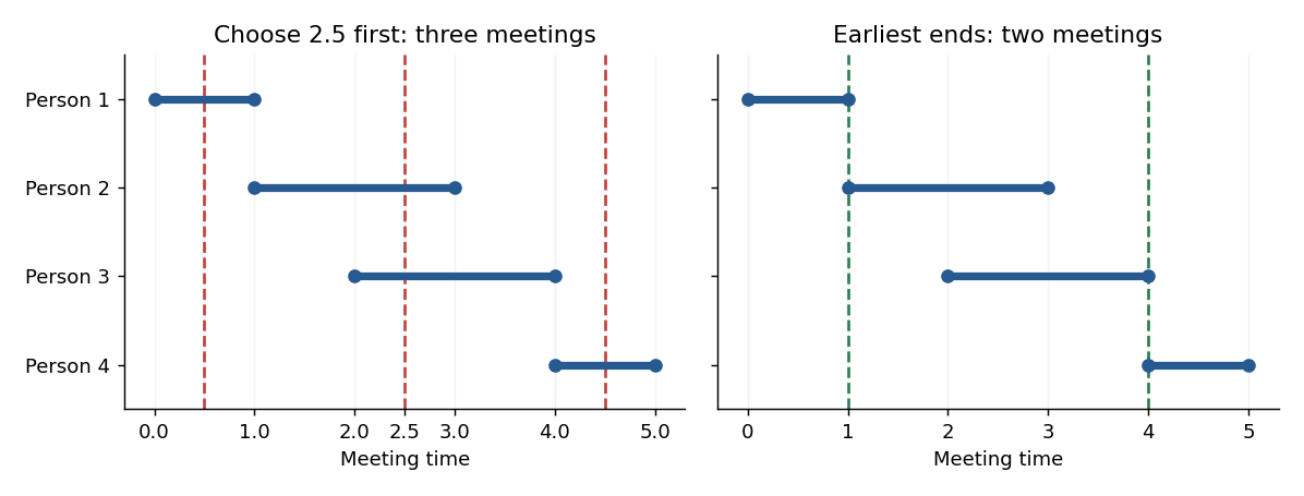
Four availability intervals: a permitted maximum-attendance choice at 2.5 leaves two extra meetings, while the endpoints 1 and 4 suffice
. **Details**.

c

Solution

The earliest end is

1

, so strategy 2 first meets at $t_{1} = 1$ , removing

I_{1}

and

I_{2}

. Among the remaining intervals the earliest end is

4

, so it next meets at $t_{2} = 4$ , removing

I_{3}

and

I_{4}

. This is the two-meeting optimum proved in part (b). The closed endpoints are essential: attendance at exactly an interval's endpoint is permitted.

d

Solution

Let

I_{i} = [s_{i}, t_{i}]

be an interval whose earliest end triggers greedy meeting

i

. After that meeting, every remaining interval starts strictly after

t_{i}

: its end is at least

t_{i}

, and otherwise it would contain

t_{i}

and be removed. Hence

s_{i + 1} > t_{i}, t_{1} < t_{2} < \dots < t_{k} .

The witness intervals

I_{1}, \dots, I_{k}

are therefore pairwise disjoint. Every feasible schedule needs a distinct meeting in each one, yielding a lower bound of

k

. The greedy schedule uses exactly

k

meetings and covers everyone, so it is optimal. This is an optimality certificate for the interval stabbing problem.

To follow the source's suggested contradiction explicitly, suppose a schedule

u_{1} < \dots < u_{j}

with

j < k

covered everyone. Since

I_{1}

ends at

t_{1}

, some

u_{ℓ} \leq t_{1}

, so

u_{1} \leq t_{1}

. If

u_{i} \leq t_{i}

and

i < j

, then none of the first

i

alternative meetings can hit

I_{i + 1}

, which starts after

t_{i}

. A later meeting must hit it by its end

t_{i + 1}

, implying

u_{i + 1} \leq t_{i + 1}

. Mathematical induction gives

u_{i} \leq t_{i}

for

1 \leq i \leq j

. But

I_{j + 1}

starts after

t_{j} \geq u_{j}

, later than every alternative meeting. It is uncovered, a contradiction. For

j = 0

a nonempty family is immediately uncovered. The source's hint starts at index zero without defining

u_{0}, t_{0}

; the proof above starts at the actual first meetings instead.

e

Solution