Past exam of the year 1 of the computer science course of the University of Oxford / 2016

Solution

For data inputs

d_{0}, \dots, d_{7}

and selection bits

s_{2} s_{1} s_{0}

, use a three-to-eight binary decoder. Its output

e_{i}

is the minterm that is one exactly when the selection equals the three-bit binary representation of

i

. For example,

e_{0} = \neg s_{2} \land \neg s_{1} \land \neg s_{0}, e_{1} = \neg s_{2} \land \neg s_{1} \land s_{0}, e_{7} = s_{2} \land s_{1} \land s_{0} .

Gate each data input with its decoded selection using an AND gate, then combine all eight results with an OR gate:

z = i = 0 ⋁ 7 (e_{i} \land d_{i}) .

Exactly one

e_{i}

is asserted, so

z = d_{i}

for the selected

i

, regardless of the other data inputs. A direct implementation uses three shared NOT gates, eight three-input AND gates for the binary decoder, eight two-input AND gates for the data, and one eight-input OR gate. Equivalently, combine each decoder term with its data input in one four-input AND gate. Larger logic gates may be built from two-input ones.

c

Solution

Use eight parallel 8:1 multiplexers and one shared three-bit binary counter. If

d_{i, j}

is bit

j

from sensor

i

, connect

d_{0, j}, \dots, d_{7, j}

to multiplexer

j

. Connect all selection inputs to the binary counter outputs. Then data line

j

carries

d_{q, j}

, so all eight data lines belong to the same selected sensor. Send the three counter outputs to the receiver as the address lines as well.

Figure 1.
One shared binary counter selects the same sensor in eight parallel multiplexers
. **Details**.

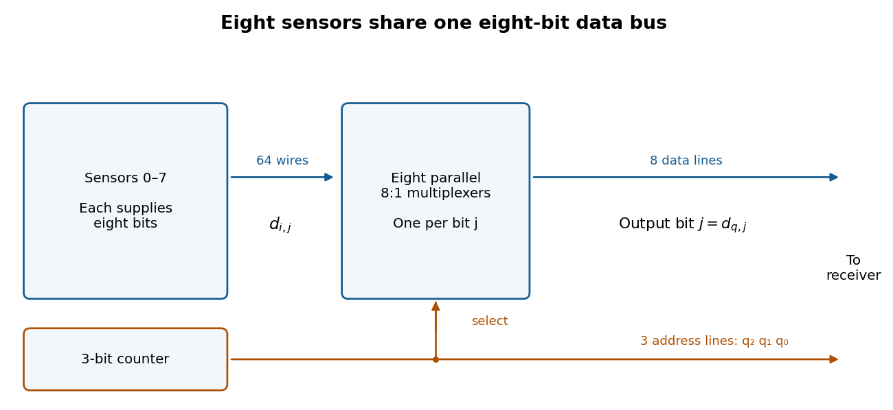
After reset the receiver sees sensors

0, 1, \dots, 7, 0, \dots

, one per clock period. Sample the data and address only after the binary counter and multiplexers have settled, for example on the opposite clock edge with a sufficiently long clock period. Changing addresses can otherwise cause transient logic hazards. The transmitter uses eleven signal lines, apart from any shared clock or reset connection.

d

Solution

Use an eight-bit modulo-256 binary counter, eight 256:1 multiplexers, eight data lines and eight address lines. Thus there are sixteen signal lines, apart from clock and reset, and a full scan takes 256 clock periods. The counter next-state equations generalize to

D_{0} = \neg q_{0}, D_{i} = q_{i} \oplus ⋀_{j = 0}^{i - 1} q_{j} (1 \leq i \leq 7) .

A 256:1 multiplexer for one data bit can be made hierarchically: 32 first-stage 8:1 multiplexers select within eight-sensor groups using

q_{2} q_{1} q_{0}

; four second-stage 8:1 multiplexers select groups using

q_{5} q_{4} q_{3}

; one final 4:1 multiplexer selects using

q_{7} q_{6}

. A final 8:1 multiplexer also works if one select input is fixed to zero and only four data inputs are used. Repeat this network eight times, sharing all selection lines. Allow for the extra propagation delay when choosing the clock period.

2

a

Solution

Generate four partial-product bits with AND gates:

p_{00} = x_{0} y_{0}, p_{10} = x_{1} y_{0}, p_{01} = x_{0} y_{1}, p_{11} = x_{1} y_{1} .

The binary multiplication expansion is

X Y = p_{00} + 2 (p_{10} + p_{01}) + 4 p_{11}

. Add the two weight-two bits with a half adder, then add its carry to

p_{11}

with a second half adder. The complete combinational logic is

z_{0} z_{2} = p_{00}, = p_{11} \oplus c, z_{1} z_{3} = p_{10} \oplus p_{01}, = p_{11} \land c . c = p_{10} \land p_{01},

Thus four AND gates for the partial products and two half adders suffice. Each half adder contains one exclusive or gate and one AND gate. In the largest case

3 \times 3 = 9

, these equations produce

1001

, including the necessary fourth output bit.

b

Solution

Split the four-bit unsigned inputs into two-bit halves:

X = 4 X_{H} + X_{L}

and

Y = 4 Y_{H} + Y_{L}

. Use four copies of the two-bit binary multiplier to compute

P_{LL} = X_{L} Y_{L}

P_{H L} = X_{H} Y_{L}

P_{L H} = X_{L} Y_{H}

, and

P_{HH} = X_{H} Y_{H}

. Then

X Y = P_{LL} + 4 P_{H L} + 4 P_{L H} + 16 P_{HH} .

The extreme terms occupy disjoint output positions:

P_{LL}

uses positions zero to three and

16 P_{HH}

uses positions four to seven. Form

W

by concatenating their four-bit outputs, with

P_{HH}

in the upper half and

P_{LL}

in the lower half. This needs wiring alone, so

W = 16 P_{HH} + P_{LL}

without an adder.

Use the first eight-bit adder to form

R = P_{H L} + P_{L H}

after zero-extension, and the second to form

Z = W + (R ≪ 2)

. Thus four two-bit binary multipliers and two eight-bit adders suffice. The fixed left bit shift is also wiring alone.

The middle sum can reach

9 + 9 = 18

, so preserve all five of its potentially nonzero bits; retaining only four would be wrong. Its shifted value is at most 72. The final result is at most

15 \times 15 = 225

, so both additions fit in eight bits. Concatenating the disjoint extreme terms is what saves an addition.

c

Solution

Use unsigned inputs as in the preceding parts. Store a 16-bit accumulator

P

, a 16-bit shifted multiplicand

M

, an eight-bit multiplier

Q

, and a three-bit iteration binary counter

k

. The sequential circuit has one 16-bit adder, a 16-bit multiplexer selecting

M

or zero from

Q_{0}

, fixed one-place bit shifts, and load/hold selection for the digital registers. The input values are captured when start is accepted, so later input changes cannot alter the operation.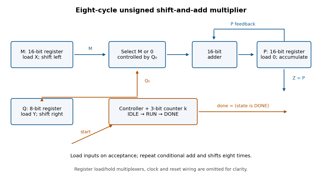

Figure 1.
The shift-and-add binary multiplier reuses one 16-bit adder for eight iterations
. **Details**.

Use three control states with the following synchronous transition table. All assignments in a row use the old digital register values and occur together at the active clock edge.

State	Condition	Register updates	Next state	IDLE	`start = 0`	Hold all digital registers	IDLE	IDLE	`start = 1`	$P \leftarrow 0$ , $M \leftarrow zeroextend_{16} (X)$ , $Q \leftarrow Y$ , $k \leftarrow 0$	RUN	RUN	$k < 7$	$P \leftarrow P + (Q_{0} ? M : 0)$ , $M \leftarrow M ≪ 1$ , $Q \leftarrow Q ≫ 1$ , $k \leftarrow k + 1$	RUN	RUN	$k = 7$	$P \leftarrow P + (Q_{0} ? M : 0)$ , $M \leftarrow M ≪ 1$ , $Q \leftarrow Q ≫ 1$ ; hold $k$	DONE	DONE	`start = 1`	Hold all digital registers	DONE	DONE	`start = 0`	Hold all digital registers	IDLE

Reset selects IDLE and clears the digital registers. Set $Z = P$ and done = 1 exactly in DONE. A start pulse in IDLE launches one multiplication; further pulses during RUN are ignored. Holding start high cannot repeatedly launch operations: DONE waits for it to go low before rearming. The product remains stored while waiting and through the following IDLE state. There are eight RUN clock edges after the loading edge; the last addition is captured before done becomes high.

For correctness, let

X_{0}, Y_{0}

denote the captured values. After

i

iterations, for

0 \leq i \leq 8

, the loop invariant is

P_{i} = X_{0} (Y_{0} mod 2^{i}), M_{i} = 2^{i} X_{0}, Q_{i} = ⌊ Y_{0} / 2^{i} ⌋,

P_{i} + M_{i} Q_{i} = X_{0} Y_{0}

. Writing

Q_{i} = 2 q + b

, the next accumulation adds

b M_{i}

, the left bit shift doubles

M_{i}

, and the logical right shift changes

Q_{i}

q

. Hence the invariant is preserved. At

i = 8

Q_{i} = 0

, giving $Z = P_{8} = X_{0} Y_{0}$ . The largest product is

25 5^{2} = 65025 < 2^{16}

, so the accumulator fits. Even the final shifted multiplicand is

256 X_{0} \leq 65280

, so it also fits.

3

a

Solution

The calling convention passes the integer argument in $a0, returns the result in $v0, and uses jal with $ra for a call and its return address. The callee returns using jr $ra. Its stack frame grows downwards from $sp and must be removed before returning, restoring the caller's stack pointer.

The $s processor registers are callee-saved registers: a callee that uses $s0 or $s1 must restore their incoming values. The $a, $v, and $t processor registers are caller-saved registers; a caller must preserve any of their values that it needs after a call. Consequently foo keeps its own argument in $s0 and the first call's result in $s1, where nested calls preserve them. Because a nested jal overwrites $ra, foo also saves its incoming return address. Every recursive activation has its own stack frame.

The supplied MIPS instructions use the paper's simplified convention: pseudoinstructions such as subi are accepted, and control transfers have no branch delay slot. The completed code below follows that convention. A hardware implementation with delayed control transfers requires suitable scheduling or nop instructions throughout the supplied code as well.

b

Solution

The entry sequence creates one 12-byte stack frame, then preserves the return address and both used callee-saved registers:

subi $sp, $sp, 12    # allocate three four-byte words
sw   $ra, 0($sp)     # save return address of this activation
sw   $s0, 4($sp)     # save caller's s0
sw   $s1, 8($sp)     # save caller's s1

The closing sequence reverses these effects:

lw   $ra, 0($sp)     # recover return address of this activation
lw   $s0, 4($sp)     # restore caller's s0
lw   $s1, 8($sp)     # restore caller's s1
addi $sp, $sp, 12    # deallocate the frame
jr   $ra            # return to the caller

Loads must precede deallocation because their offsets refer to the current stack frame. The return value in $v0 is deliberately retained. Saving $ra is essential even though it is not an $s processor register: otherwise the second nested call would destroy the address to which this activation must return.

c

Solution

The missing MIPS instructions, in order, are

bne  $t0, $0, fooRet1
subi $a0, $s0, 3
add  $v0, $s1, $v0

The comparison slti $t0, $s0, 3 makes $t0 nonzero exactly when

y < 3

, so the first instruction selects the base case. The second forms

y - 3

from the saved argument, rather than relying on $a0 surviving the first call. After the second call, $s1 holds bar(y-2) and $v0 holds bar(y-3); the final addition puts their sum in $v0, as required by the calling convention.

d

Solution

The blanks are x < 2 and return x - foo(x + 1). The compiled slti and bne select the first branch exactly for

x < 2

. Otherwise addi forms

x + 1

, jal foo returns its value in $v0, and sub $v0, $s0, $v0 subtracts that value from the preserved

x

. Thus the complete high-level implementation is

proc bar(val x : int) : int
begin if x < 2 then
          return 1
      else
          return x - foo(x + 1)
      end
end

Although the immediate call increases the argument, substitution into foo's two recursive calls decreases the corresponding bar arguments to

x - 1

and

x - 2

whenever the recursive branch is entered. The mutual recursion therefore terminates on ordinary integer inputs, assuming sufficient stack space and no machine arithmetic overflow.

e

Solution

Keep both the limit and current argument in callee-saved registers, so a call to foo preserves them. Under the same no-delay-slot convention, use

li   $s0, n
li   $s1, 1
slti $t0, $s0, 1
bne  $t0, $0, testEnd
testLoop:
move $a0, $s1
jal  foo
break 1
beq  $s1, $s0, testEnd
addi $s1, $s1, 1
b    testLoop
testEnd:
break 0
b    testEnd

At every break 1, $s1 is the tested value and $v0 is its result. Resuming after the breakpoint continues to the next value; after

n

the program reaches its separate final stop. The initial guard handles

n < 1

with no calls. Testing equality before incrementing also avoids overflowing the loop variable after the final call when

n

is the largest positive machine integer. As with the supplied procedures, evaluating all calls assumes enough stack space and representable arithmetic results.

4

a

Solution

The third left-hand side is three times the first minus the second. Consistency of this linear system therefore requires

2 = 3 a - a^{2}

, or

a^{2} - 3 a + 2 = (a - 1) (a - 2) = 0.

This is also sufficient: the first two rows are linearly independent, and on setting the free variable

x_{3} = t

they give

a \in {1, 2}, (x_{1}, x_{2}, x_{3}) = (a - t, a^{2} - 2 a - 3 t, t), t \in R .

Substitution into the third equation gives

3 a - a^{2} = 2

for either allowed

a

. Explicitly the solution families are

(1 - t, - 1 - 3 t, t)

and

(2 - t, - 3 t, t)

. For every other

a

, the same row relation gives an immediate inconsistency.

b

Solution

Denote the columns by

c_{1}, \dots, c_{4}

. The first two are linearly independent, because the top two coordinates have determinant

3 \cdot 2 - (- 1) \cdot 1 = 7

. Direct calculation gives

c_{3} = \frac{1}{7} c_{1} - \frac{4}{7} c_{2}, c_{4} = \frac{5}{7} c_{1} + \frac{1}{7} c_{2} .

Thus a column-space basis is ${(3, 1, 9)^{T}, (- 1, 2, 4)^{T}}$ , and

Col (A) = span {c_{1}, c_{2}} = {(u, v, 2 u + 3 v)^{T} : u, v \in R} .

For the last description, the third row equals twice the first row plus three times the second, so every column lies in that plane. Since the two independent columns already span a two-dimensional vector subspace, they fill the plane.

The target vector satisfies

5 = 2 (- 2) + 3 (3)

, so it is in the column space. An especially simple linear combination is

b = c_{2} - c_{3} = (- 1, 2, 4)^{T} - (1, - 1, - 1)^{T} = (- 2, 3, 5)^{T} .

(3)

In terms of the displayed basis, the same vector is

- c_{1} /7 + 11 c_{2} /7

. The column space itself is unique; the freedom is in choosing its basis.

c

Solution

No. Take the one-by-one matrices

A = [1]

B = [- 1]

. Both column spaces are

C = R

, whereas

A + B = [0]

has column space

{0}

. More generally, taking

B = - A

cancels any nonzero column space. One always has

Col (A + B) \subseteq C

, because each sum column lies in the vector subspace

C

, but equality can fail through cancellation.

5

a

Solution

For square matrices of the same size,

det (A B) = det (A) det (B) .

For an upper or lower triangular matrix

T

, its determinant is the product of its diagonal entries:

det (T) = i = 1 \prod n t_{ii} .

These formulas include singular matrices and zero diagonal entries.

b

Solution

Let

e_{i}

be standard coordinate columns. The required elementary matrix is

E = I_{n} + α e_{j} e_{i}^{T}, E A : R_{j} \leftarrow R_{j} + α R_{i} .

It is the identity matrix with the extra entry

α

in position

(j, i)

. Left matrix multiplication implements the row operation: all other rows are unchanged. Since

j > i

E

is a lower triangular matrix with every diagonal entry one. Part (a) therefore gives

det (E) = 1

and

det (E A) = det (E) det (A) = det (A) .

Hence adding a multiple of one row to another leaves the determinant unchanged, even if

A

is singular.

c

Solution

Use

- A = (- I_{n}) A

. The diagonal matrix

- I_{n}

has

n

diagonal entries equal to

- 1

, so the product and triangular matrix formulas from part (a) give

det (- A) = det (- I_{n}) det (A) = (- 1)^{n} det (A) .

Equivalently, multiplying each of the

n

rows by

- 1

supplies one factor

- 1

per row.

d

Solution

Write the determinant in its Leibniz formula for determinants, where

S_{n}

is the set of permutations of

{1, \dots, n}

det (A) = \sum_{σ \in S_{n}} sgn (σ) \prod_{i = 1}^{n} a_{i, σ (i)} .

The permutation sign is justified by the given row-interchange property: a permutation matrix is obtained from the identity matrix by row interchanges, and every interchange changes its determinant by a factor

- 1

. Reversing a sequence of interchanges constructs the inverse permutation with the same number of interchanges. Consequently

sgn (σ^{- 1}) = sgn (σ)

. The Leibniz formula for determinants can itself be obtained by expanding the rows multilinearly in the standard basis: repeated selected coordinate rows contribute zero, and the remaining terms are precisely these signed permutation matrices.

Since

(A^{T})_{ij} = a_{ji}

, the same formula gives

det (A^{T}) = \sum_{σ \in S_{n}} sgn (σ) \prod_{i = 1}^{n} a_{σ (i), i} .

Reindex the product with

j = σ (i)

and reindex the sum with

τ = σ^{- 1}

. Both reindexings are bijections, so

det (A^{T}) = \sum_{τ \in S_{n}} sgn (τ) \prod_{j = 1}^{n} a_{j, τ (j)} = det (A) .

(3)

Thus $det (A) = det (A^{T})$ for every real square matrix, including singular matrices. This proof does not assume the analogous column-operation rules in order to establish the transpose identity.

e

Solution

For a skew-symmetric matrix,

A^{T} = - A

. By parts (c) and (d),

det (A) = det (A^{T}) = det (- A) = (- 1)^{n} det (A) .

n

is odd,

det (A) = - det (A)

, hence

2 det (A) = 0

over

R

. Therefore $det (A) = 0$ , so $A$ is a singular matrix. The conclusion depends on odd dimension: in dimension two,

(0 - 1 10)

is skew-symmetric and has determinant one.

6

a

Solution

An eigenvalue and eigenvector pair

(λ, v)

for a square matrix

A

satisfies

A v = λ v, v \neq = 0.

The scalar

λ

and the coordinates of

v

belong to the chosen field, usually

R

C

. The nonzero condition is essential: the zero vector satisfies the equation for every

λ

and therefore cannot define an eigenvalue.

b

Solution

The vectors

v_{1}, \dots, v_{n}

are linearly independent if

α_{1} v_{1} + \dots + α_{n} v_{n} = 0 ⟹ α_{1} = \dots = α_{n} = 0.

They are linearly dependent if some such relation has at least one nonzero coefficient. All coefficients lie in the underlying field. Thus linear independence means that only the trivial linear combination gives zero; linear dependence means that a nontrivial one does.

c

Solution

Apply

A

to the stated linear combination and use each eigenvector equation:

λ_{k + 1} z_{k + 1} = A z_{k + 1} = \sum_{i = 1}^{k} α_{i} A z_{i} = \sum_{i = 1}^{k} α_{i} λ_{i} z_{i} .

Subtract

λ_{k + 1}

times the original relation. This gives

\sum_{i = 1}^{k} α_{i} (λ_{i} - λ_{k + 1}) z_{i} = 0.

The assumed linear independence implies

α_{i} (λ_{i} - λ_{k + 1}) = 0

separately for every

i

. Since the eigenvector

z_{k + 1}

is nonzero, not all

α_{i}

can vanish. Choose any

i

with

α_{i} \neq = 0

; division by that coefficient gives $λ_{i} = λ_{k + 1}$ . In fact every nonzero coefficient is attached to that same eigenvalue.

d

Solution

Interpret “distinct eigenvalues” as $n$ pairwise distinct eigenvalues in the chosen field. Select a nonzero eigenvector

z_{i}

for each. A single nonzero vector is linearly independent. Suppose inductively that

z_{1}, \dots, z_{k}

are linearly independent. If adding

z_{k + 1}

made the set linearly dependent, its nontrivial relation would have a nonzero coefficient of

z_{k + 1}

, since otherwise it would contradict the induction hypothesis. Solving for

z_{k + 1}

would place it in the linear span of the first

k

eigenvectors.

Part (c) would then force

λ_{k + 1} = λ_{i}

for some

i \leq k

, contradicting pairwise distinctness. Mathematical induction therefore proves that all $n$ selected eigenvectors are linearly independent, forming a basis. If the field is

R

, the assertion requires

n

real eigenvalues; a real matrix can instead have nonreal eigenvalues and a eigenvector basis over the complex numbers.

e

Solution

For

A

, the triangular matrix formula gives the characteristic polynomial

det (t I - A) = (t - 1) (t - 3) (t - 2) .

The three eigenvalues are distinct, so part (d) already proves the existence of an eigenvector basis. Explicit choices, ordered by eigenvalues

1, 3, 2

, are

(1, 0, 0)^{T}, (1, 1, 0)^{T}, (2, - 1, 1)^{T} .

Their column matrix has determinant one, and direct multiplication gives respectively one, three and two times the indicated vector.

For

B

, expansion along the last row gives

det (t I - B) = (t - 3) ((t - 3)^{2} - 1) = (t - 3) (t - 4) (t - 2) .

(3)

Again the three eigenvalues are distinct. An explicit eigenvector basis, ordered by eigenvalues

4, 2, 3

, is

(1, 1, 0)^{T}, (1, - 1, 0)^{T}, (0, - 1, 1)^{T} .

(4)

Its column matrix has determinant

- 2 \neq = 0

. In particular,

B

's diagonal entries are not its eigenvalues: it is not a triangular matrix.

Finally

C = I_{3}

, so every nonzero vector is an eigenvector with eigenvalue one. Choose the standard basis $e_{1}, e_{2}, e_{3}$ . These are linearly independent even though their eigenvalues coincide. Distinct eigenvalues are sufficient for an eigenvector basis, and are not necessary.

7

a

Solution

The implication introduction rule opens a subproof with a temporary assumption

ϕ

, derives

ψ

, and discharges that assumption to conclude $ϕ \to ψ$ . The negation introduction rule opens a subproof with a temporary assumption

ϕ

, derives logical falsity

⊥

, and discharges it to conclude $\neg ϕ$ .

The boxes record the scopes and dependencies of the temporary assumptions. A result derived inside a box cannot be used outside it without the appropriate discharge rule; it may depend on the boxed assumption. Other, surrounding assumptions remain in force. This is how the natural deduction rules distinguish a conditional derivation from an unconditional assertion.

b

Solution

Let

H = (P \land Q) \lor (P \land R)

. In the following natural deduction proofs, indentation and vertical bars mark assumption scopes. Rule names are the introduction and elimination rules supplied by the paper.

First work backwards from the premise using disjunction elimination, proving the whole desired logical conjunction in each case:

1  H               premise
 2  | P ∧ Q        assumption
 3  | P            ∧-elim-L 2
 4  | Q            ∧-elim-R 2
 5  | Q ∨ R        ∨-intro-L 4
 6  | P ∧ (Q ∨ R)  ∧-intro 3,5
 7  | P ∧ R        assumption (new case)
 8  | P            ∧-elim-L 7
 9  | R            ∧-elim-R 7
10  | Q ∨ R        ∨-intro-R 9
11  | P ∧ (Q ∨ R)  ∧-intro 8,10
12  P ∧ (Q ∨ R)    ∨-elim 1,2–6,7–11

Alternatively, first transform the goal by conjunction introduction, obtaining

P

and

Q \lor R

by separate disjunction elimination proofs:

1  H             premise
 2  | P ∧ Q      assumption
 3  | P          ∧-elim-L 2
 4  | P ∧ R      assumption (new case)
 5  | P          ∧-elim-L 4
 6  P            ∨-elim 1,2–3,4–5
 7  | P ∧ Q      assumption
 8  | Q          ∧-elim-R 7
 9  | Q ∨ R      ∨-intro-L 8
10  | P ∧ R      assumption (new case)
11  | R          ∧-elim-R 10
12  | Q ∨ R      ∨-intro-R 11
13  Q ∨ R        ∨-elim 1,7–9,10–12
14  P ∧ (Q ∨ R)  ∧-intro 6,13

The essential difference is the final rule: the first proof splits the premise once, while the second splits the goal first and then analyzes the premise twice. Counting only rule applications, both displayed proofs take nine inference steps. The first uses four conjunction elimination steps, two disjunction introduction steps, two conjunction introduction steps and one disjunction elimination; the second replaces one conjunction introduction with a second disjunction elimination. If assumption lines are counted as displayed proof lines, the second is longer, 14 rather than 12, because it opens four case assumptions rather than two. Thus a raw line count and an inference-step count need not agree.

c

Solution

Proof by contradiction, or reductio ad absurdum, has the form

\frac{Γ , \neg ϕ ⊢ ⊥}{Γ ⊢ ϕ} RAA,

discharging the assumption

\neg ϕ

. This is the classical rule that concludes

ϕ

directly, as opposed to the negation introduction rule, which concludes a negation.

To derive double-negation elimination using RAA without assuming double-negation elimination itself, use

1  ¬¬φ   premise
2  | ¬φ  assumption
3  | ⊥   ¬-elim 2,1
4  φ     RAA 2–3

Here line 1 is the negation of line 2. Thus only negation elimination rule inside the subproof, followed by RAA, is needed.

d

i

Solution

Abbreviate

H = (\neg P) \to Q

and

K = (\neg P) \to \neg Q

. Use the primitive natural deduction rules, including double-negation elimination:

1  H             premise
 2  | H          assumption
 3  | | K        assumption
 4  | | | ¬P     assumption
 5  | | | Q      →-elim 2,4
 6  | | | ¬Q     →-elim 3,4
 7  | | | ⊥      ¬-elim 5,6
 8  | | ¬¬P      ¬-intro 4–7
 9  | | P        ¬¬-elim 8
10  | K → P      →-intro 3–9
11  H → (K → P)  →-intro 2–10

The outer premise is redundant: the proof uses the locally assumed

H

, so the conclusion is already a theorem. Keeping the redundant premise is allowed. The successive discharges give $((\neg P) \to Q) \to (((\neg P) \to \neg Q) \to P)$ with exactly the requested assumption scopes.

ii

Solution

First derive

A

by double-negation elimination, then derive

\neg B

by negation introduction. The logical falsity elimination rule is used only inside the attempt to derive

A

1  ¬(A → B)  premise
 2  | ¬A     assumption
 3  | | A    assumption
 4  | | ⊥    ¬-elim 3,2
 5  | | B    ⊥-elim 4
 6  | A → B  →-intro 3–5
 7  | ⊥      ¬-elim 6,1
 8  ¬¬A      ¬-intro 2–7
 9  A        ¬¬-elim 8
10  | B      assumption
11  | | A    assumption
12  | | B    reiteration 10
13  | A → B  →-intro 11–12
14  | ⊥      ¬-elim 13,1
15  ¬B       ¬-intro 10–14
16  A ∧ ¬B   ∧-intro 9,15

Reiteration at line 12 merely uses an assumption that remains in scope. The final $A \land \neg B$ follows by conjunction introduction. This explicitly supplies the classical step needed to obtain

A

rather than just

\neg\neg A

8

a

i

Solution

Use negation introduction on the unwanted existential quantification, and existential quantifier elimination rule with a fresh witness

a

1  ∀x. ¬P(x)    premise
2  | ∃x. P(x)   assumption
3  | | P(a)     assumption, a fresh
4  | | ¬P(a)    ∀-elim 1
5  | | ⊥        ¬-elim 3,4
6  | ⊥          ∃-elim 2,3–5
7  ¬(∃x. P(x))  ¬-intro 2–6

The witness name occurs neither in the surrounding assumptions nor in the conclusion

⊥

of its subproof. This satisfies the eigenvariable condition; it is not an arbitrarily chosen fixed element assumed to witness the existential quantification. The result is $\neg\exists x P (x)$ .

ii

Solution

Choose a fresh parameter

a

. The universal quantifier elimination rule supplies both the implication and its premise at that same parameter:

1  ∀x. (P(x) → Q(x))        premise
2  | ∀x. P(x)               assumption
3  | P(a)                   ∀-elim 2
4  | P(a) → Q(a)            ∀-elim 1
5  | Q(a)                   →-elim 4,3
6  | ∀x. Q(x)               ∀-intro 5, a fresh
7  (∀x. P(x)) → (∀x. Q(x))  →-intro 2–6

The eigenvariable condition holds because

a

is absent from both undischarged assumptions at line 6. Hence the universally quantified implication is proved.

The proposed version with merely

P (x)

in the antecedent is not derivable. For a counterexample, take a two-element domain

{0, 1}

with

P

and

Q

both true precisely at zero. The universal premise holds. Under the assignment

x = 0

P (x)

is true but

\forall x Q (x)

is false. By soundness, a formal proof cannot exist. Attempting the previous derivation would fail exactly at universal quantifier introduction rule: the parameter would occur in the undischarged assumption

P (x)

, so it would not be fresh.

b

Solution

Write

H (t) = \forall p ((S (t, p) \to \neg S (p, p)) \land (\neg S (p, p) \to S (t, p)))

. Use negation introduction on the existential claim. For its fresh witness

b

, instantiate

p = b

; the resulting self-application says both

S (b, b) \to \neg S (b, b)

and its reverse. The given law of excluded middle then provides the two cases.

1  ∀x. ∀y. (S(x,y) ∨ ¬S(x,y))                    premise
 2  | ∃b. H(b)                                   assumption
 3  | | H(b)                                     assumption, b fresh
 4  | | (S(b,b) → ¬S(b,b)) ∧ (¬S(b,b) → S(b,b))  ∀-elim 3, p := b
 5  | | S(b,b) → ¬S(b,b)                         ∧-elim-L 4
 6  | | ¬S(b,b) → S(b,b)                         ∧-elim-R 4
 7  | | ∀y. (S(b,y) ∨ ¬S(b,y))                   ∀-elim 1, x := b
 8  | | S(b,b) ∨ ¬S(b,b)                         ∀-elim 7, y := b
 9  | | | S(b,b)                                 assumption
10  | | | ¬S(b,b)                                →-elim 5,9
11  | | | ⊥                                      ¬-elim 9,10
12  | | | ¬S(b,b)                                assumption (new case)
13  | | | S(b,b)                                 →-elim 6,12
14  | | | ⊥                                      ¬-elim 13,12
15  | | ⊥                                        ∨-elim 8,9–11,12–14
16  | ⊥                                          ∃-elim 2,3–15
17  ¬∃b. H(b)                                    ¬-intro 2–16

Both case assumptions are discharged at line 15; the witness assumption is discharged at line 16. Since

b

is absent from the surrounding premise and the exported conclusion

⊥

, existential quantifier elimination rule is valid. Line 17 is the required negated existential. This is the diagonal self-application underlying the barber paradox.

c

i

Solution

Equality introduction rule is reflexivity; equality elimination rule permits substitution of equals in a formula:

Γ ⊢ t = t (= I), \frac{Γ ⊢ s = t Γ ⊢ ϕ ( s )}{Γ ⊢ ϕ ( t )} (= E) .

Terms substituted into

ϕ

must be free for substitution, so no variable becomes captured. The notation

ϕ (s), ϕ (t)

means substitution into the same designated free variable positions of one formula; other occurrences may remain fixed. These rules express first-order equality without assuming symmetry or transitivity as additional axioms.

ii

Solution

For transitivity of first-order equality, take the substitution formula

ϕ (u) \equiv (T_{1} = u)

1  T₁ = T₂  premise
2  T₂ = T₃  premise
3  T₁ = T₃  =-elim 2,1; φ(u) := (T₁ = u)

For symmetry, use reflexivity and

ψ (u) \equiv (u = T_{1})

1  T₁ = T₂  premise
2  T₁ = T₁  =-intro
3  T₂ = T₁  =-elim 1,2; ψ(u) := (u = T₁)

Thus both transitivity and symmetry follow from the two equality rules. In the symmetry proof, only the designated first occurrence in

T_{1} = T_{1}

is replaced; the second remains fixed.

iii

Solution

Choose distinct fresh parameters

a, b

. Within the assumption

a = b

, equality elimination rule gives the forward implication directly. Derive the reverse equality explicitly before using it for the reverse implication:

1  | a = b                                           assumption
 2  | | P(a)                                         assumption
 3  | | P(b)                                         =-elim 1,2
 4  | P(a) → P(b)                                    →-intro 2–3
 5  | a = a                                          =-intro
 6  | b = a                                          =-elim 1,5; φ(u) := (u = a)
 7  | | P(b)                                         assumption
 8  | | P(a)                                         =-elim 6,7
 9  | P(b) → P(a)                                    →-intro 7–8
10  | (P(a) → P(b)) ∧ (P(b) → P(a))                  ∧-intro 4,9
11  a = b → ((P(a) → P(b)) ∧ (P(b) → P(a)))          →-intro 1–10
12  ∀y. a = y → ((P(a) → P(y)) ∧ (P(y) → P(a)))      ∀-intro 11, b fresh
13  ∀x. ∀y. x = y → ((P(x) → P(y)) ∧ (P(y) → P(x)))  ∀-intro 12, a fresh

The equality assumption is discharged before either universal quantifier introduction rule. There are then no undischarged assumptions, so both eigenvariable condition requirements hold. The final universal theorem expresses that equal arguments are interchangeable in the predicate

P

in both directions.

Digital systems, linear algebra, introduction to formal proof (resit) (A10101W1)

Source paper: released examination archive, member a10101w1-2.pdf; original cover dated 2016-09-15.

1

a

Solution

Take

w, x, y, z

as the four input bits, of weights

8, 4, 2, 1

, and let 1 light a segment of the seven-segment display. The required truth table is

value   wxyz   abcdefg
 0      0000   1111110
 1      0001   0110000
 2      0010   1101101
 3      0011   1111001
 4      0100   0110011
 5      0101   1011011
 6      0110   1011111
 7      0111   1110000
 8      1000   1111111
 9      1001   1111011
10      1010   0000000
11      1011   0000000
12      1100   0000000
13      1101   0000000
14      1110   0000000
15      1111   0000000

Here binary-coded decimal represents one decimal digit per group of four bits. The six unused codes must be zeros in every output for this part; they are not don't-care conditions.

b

Solution

Use Karnaugh maps with rows

w x

and columns

yz

, both in Gray code order

00, 01, 11, 10

. Juxtaposition means Boolean conjunction,

+

means Boolean disjunction, and a bar means Boolean negation. The minimal sum of products forms are

c = \overset{w}{ˉ} x + \overset{w}{ˉ} z + \overset{x}{ˉ} \overset{y}{ˉ},

and

d = w \overset{x}{ˉ} \overset{y}{ˉ} + \overset{w}{ˉ} \overset{x}{ˉ} y + \overset{w}{ˉ} y \overset{z}{ˉ} + \overset{w}{ˉ} \overset{x}{ˉ} \overset{z}{ˉ} + \overset{w}{ˉ} x \overset{y}{ˉ} z .

For

c

, the groups are

{4, 5, 6, 7}

{1, 3, 5, 7}

and

{0, 1, 8, 9}

. For

d

, take

{8, 9}

{2, 3}

{2, 6}

{0, 2}

and the isolated minterm

{5}

. Every group contains only required ones. The last

c

group wraps between the top and bottom map rows.

These covers are minimal:

c

needs its three essential groups, forced by inputs 6, 3 and 8. For

d

, input 5 is isolated, while 9, 3 and 6 each force their respective pair; input 0 still needs a further group. These five groups also attain the minimum literal count of 16.

Figure 1.
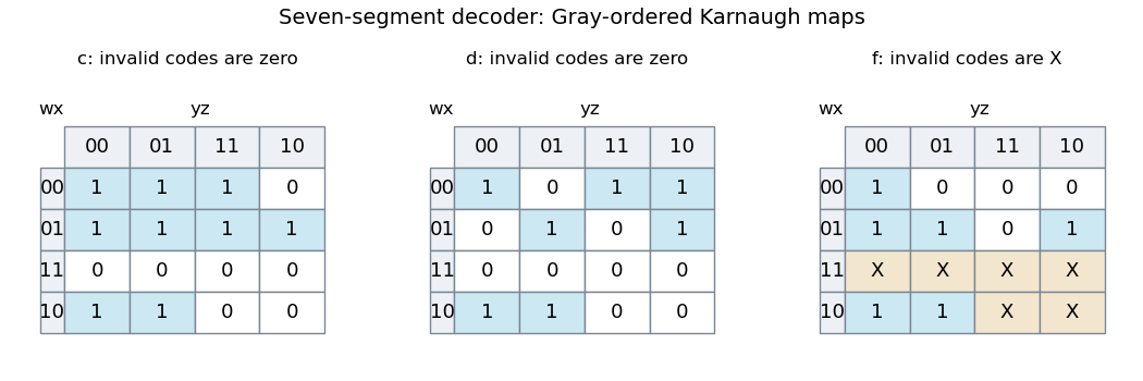
Karnaugh maps for the three decoder outputs used in the solution
. Original maps in Gray order. Invalid inputs are fixed to zero for $c$ and $d$ ; only the $f$ map in part (d) treats them as X. Blue cells are required ones. **Details**.

c

Solution

Use

w, x, y

as the three select bits of the 8-to-1 multiplexer, so address

i = 4 w + 2 x + y

selects data input

D_{i}

. Connect

(D_{0}, D_{1}, D_{2}, D_{3}, D_{4}, D_{5}, D_{6}, D_{7}) = (\overset{z}{ˉ}, 1, z, \overset{z}{ˉ}, 1, 0, 0, 0) .

A single NOT gate produces

\overset{z}{ˉ}

, shared by

D_{0}

and

D_{3}

; the other connections are wires and constant logic levels. For each fixed select address the data input reproduces the corresponding two rows of the truth table, including zeros for all invalid codes.

d

Solution

Only now may the invalid codes 10–15 be marked as don't-care conditions. The

f

Karnaugh map gives

f = w + x \overset{y}{ˉ} + x \overset{z}{ˉ} + \overset{y}{ˉ} \overset{z}{ˉ} .

The groups are

{8, \dots, 15}

{4, 5, 12, 13}

{4, 6, 12, 14}

and

{0, 4, 8, 12}

. They cover all required ones, avoid valid-digit zeros, and may assign either output to invalid codes. The valid inputs 0, 5, 6 and 9 cannot share a valid implicant with each other, so at least four product terms are necessary. The displayed four-term cover uses only seven literals.

2

a

Solution

Use a four-state Moore machine. In state

A

wait for an outer-sensor activation;

B

combines the outer-only and both-sensors phases;

C

records that the visitor has reached the inner-only phase;

I

emits the one-cycle count pulse. Only

I

has INC = 1.

The complete state transition table, with input order

x_{1} x_{0}

, is

state    00    01    11    10    INC
 A        A     B     B     A      0
 B        A     B     B     C      0
 C        I     B     B     C      0
 I        A     B     B     A      1

For a normal entry the states are

A \to B \to B \to C \to I

; retreat after the first sensor instead gives

A \to B \to A

with no pulse. Repeated samples at one sensor remain in the corresponding phase. State

I

always exits on the next edge, so its output lasts exactly one clock period; an outer activation on that next edge goes directly to

B

, allowing the next visitor to start immediately.

This follows the question's single-visitor entry model and merges the two outer-active phases as its hint requests. Inputs are sampled synchronously; the table also specifies deterministic recovery for other sampled combinations. It is not a specification of a bidirectional occupancy counter for arbitrary overlapping entry and exit traffic.

Figure 1.
Four-state visitor-entry Moore machine with a one-clock output pulse
. Original state diagram. Edge labels use $x_{1} x_{0}$ . State I emits the count pulse; its transitions can accept the next visitor without an extra idle clock. **Details**.

b

Solution

Encode

(q_{1} q_{0})

A = 00

B = 01

C = 11

I = 10

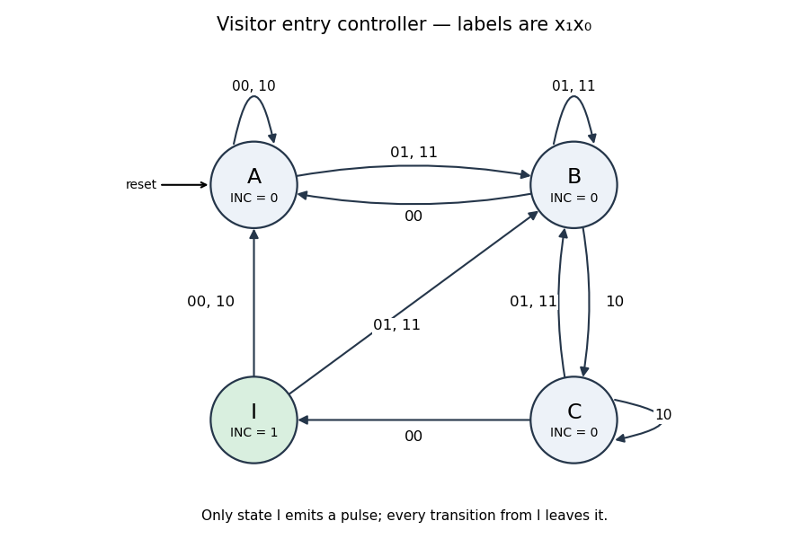
, with reset to

A

. Two positive-edge-triggered D flip-flops store the state. Minimizing the Boolean functions from the complete table gives

D_{0} = x_{0} + q_{0} x_{1}, D_{1} = \overset{x}{ˉ}_{0} q_{0} (x_{1} + q_{1}), I NC = q_{1} \overset{q}{ˉ}_{0} .