Solutions for all eight questions of the 5 September 2022, three-hour resit in the Year 1 of the computer science course of the University of Oxford. The cover date identifies this paper despite the archive member being filed under
2021/L.Public source: Oxford-supplied archive, member 2021/L/a10097w1.pdf.[ref]
Functional programming, design and analysis of algorithms, Long Vacation 2022 by University of Oxford. Cover, formal code A10097W1; original pages 2–8
For finite lists, use structural induction: establish
P []; then, for arbitrary x and xs, assume P xs and prove P (x:xs). The induction hypothesis must quantify over any other parameters that need to change in the step.For all Haskell list values, finite terminating spines are insufficient: also establish
P undefined, and allow arbitrary, possibly undefined, heads in the cons step. This proves the equation for finite partial lists ending in the bottom value. An infinite lazy list is the limit of these finite approximations. Equations between pure definable computable functions are preserved by those limits, so the equation extends to infinite inputs. This last argument requires that admissibility property; an arbitrary logical property of lists need not have it. The distinction between [] and the bottom value is essential.[ref]Take compatible function types
f :: b -> c, g :: b -> a -> b, and h :: c -> a -> c. The necessary conditions obtained from the two induction base cases are strictness of f and the fusion equationAt zs = [], the desired equation is exactly the displayed fusion equation. At zs = undefined, both left folds diverge because their list argument has no outer constructor; the equation therefore requires f undefined = undefined. This is the strict function condition. If only finite total spines were considered, the first condition would not be necessary.These conditions also support the step. The induction hypothesis must hold for every accumulator and element. For The middle rewrite uses the fusion equation at
z:zs, instantiate that hypothesis at g x y and z:f (foldl g (g x y) (z:zs))
= f (foldl g (g (g x y) z) zs)
= foldl h (h (f (g x y)) z) zs
= foldl h (h (h (f x) y) z) zs
= foldl h (h (f x) y) (z:zs).x,y. For pure computable functions, equality on infinite spines follows from finite approximations as in part (a).Prove the stronger equation, quantified over the accumulator:For Thus structural induction proves the claim for finite and finite partial spines; definable continuity extends it to infinite lazy lists. Pointwise equality is exactly the asserted equality of function compositions. This is the left-fold fusion law.
[], both sides are f a. For the bottom value, both sides are bottom because f is a strict function. For the cons step, the universal induction hypothesis allows the accumulator to become g a x:f (foldl g a (x:xs))
= f (foldl g (g a x) xs)
= foldl h (f (g a x)) xs
= foldl h (h (f a) x) xs
= foldl h (f a) (x:xs).Use a type with distinct values Since
a and n, and let s _ y = y. Suppose a direct right fold with the same result type represented this left fold. The empty list forces k = n. The singleton lists force c n n = n and c a n = a. But thenfoldr c k [a,n] = c a (c n n) = c a n = a,
foldl s n [a,n] = n.a /= n, this is a counterexample. A direct right fold cannot recover whether its tail result n came from the empty list or from the singleton [n]. The obstruction already occurs on finite total inputs, so it also rules out an implementation valid on all lazy lists.Change the right fold's result type to an accumulator-transforming function type:Thus
foldlAsFoldr :: (b -> a -> b) -> b -> [a] -> b
foldlAsFoldr s n xs = foldr c id xs n
  where
c x k a = k (s a x)c x k = \a -> k (s a x) and k = id in the question's notation. Here c :: a -> (b -> b) -> (b -> b), and the fold's base value is the identity function, not the initial accumulator n.The recursion invariant is At an undefined spine, applying the undefined folded function also gives the bottom value. The finite-approximation argument then covers infinite lazy lists. This is a continuation representation of a left fold: the result retains the operation still to be performed, avoiding the information loss in part (d).
foldr c id xs a = foldl s a xs for every a. For [], both sides equal a. For a cons:foldr c id (x:xs) a
= c x (foldr c id xs) a
= foldr c id xs (s a x)
= foldl s (s a x) xs
= foldl s a (x:xs).A value-bearing perfect binary tree has size , and the next size is . Suppose two size- trees have at least one smaller tree before them. The portion represented by these trees and that nonempty preceding portion has at least elements. The greedy choice would have used a larger perfect binary tree instead, contradicting the specified representation. Three size- trees are likewise impossible, since . Therefore the only possible repeated size is a pair at the beginning. This is the representation invariant of a skew-binary random-access list.
A Haskell representation is:Every tree stores a value at its root, including internal nodes. Interpret the forest by root-left-right preorder traversal, concatenating the results in forest order. Valid values have correct cached sizes, perfect binary trees, nondecreasing sizes and only the permitted initial duplicate. The raw constructors can express invalid representations, so the operations below assume valid values and should form the public interface. Sizes are assumed to fit in
import Prelude hiding (null, head, tail)

data RTree a = Leaf a | Node a (RTree a) (RTree a)
newtype List a = List [(Int, RTree a)]Int; the stated time complexities use constant-time size arithmetic.The empty skew-binary random-access list contains no trees:Both construction of
nil :: List a
nil = List []

null :: List a -> Bool
null (List []) = True
null _ = Falsenil and testing null take constant time.Only the first two trees need inspection:When the first sizes agree, place
cons :: a -> List a -> List a
cons x (List ((w,t):(v,u):ts))
  | w == v = List ((2*w+1, Node x t u):ts)
cons x (List ts) = List ((1, Leaf x):ts)x above those two perfect binary trees. Its preorder traversal is x followed by the old two traversals. No further size- tree can occur, so all remaining sizes are at least ; equality creates at most the allowed initial duplicate. When the first sizes differ, adjoining a singleton is valid, including the case that the old first tree is also a singleton. These are exactly the two possible greedy representations after increasing the length by one. Each case creates a bounded number of constructors and inspects no tree interior, giving worst-case time complexity. Existing trees are shared.Repeated constant time insertion constructs the representation:The right fold preserves order because
fromList :: [a] -> List a
fromList = foldr cons nilcons prepends its argument. On a finite length- list, there are calls of cons; completely constructing the result takes time and constructors. This claim concerns finite inputs, not productivity of conversion from an infinite lazy list.The first tree's root is the first element. Deleting that root either discards a singleton or exposes two equal-sized child trees:For a node of size , both children have size . Their order agrees with the old preorder traversal, and they become the sole permitted initial duplicate. The rest of the forest was no smaller than the old root tree. Thus both operations preserve the representation invariant and take worst-case time on a nonempty skew-binary random-access list.
head :: List a -> a
head (List ((_,Leaf x):_))     = x
head (List ((_,Node x _ _):_)) = x
head (List []) = error "head: empty list"

tail :: List a -> List a
tail (List ((_,Leaf _):ts)) = List ts
tail (List ((w,Node _ l r):ts)) =
  let h = w `div` 2 in List ((h,l):(h,r):ts)
tail (List []) = error "tail: empty list"Repeated root removal gives the conventional list:The representation interpretation satisfies
toList :: List a -> [a]
toList rs
  | null rs   = []
| otherwise = head rs : toList (tail rs)toList (cons x rs) = x : toList rs; alternatively, structural induction on the number of stored elements proves that each step emits exactly the next preorder traversal value. The output has cons cells, and each step takes constant time, so fully consuming it costs time. No repeated list concatenation is needed.Skip whole trees using their cached sizes, then descend through one tree:After skipping a size- tree, the desired index decreases by . Inside a node, position zero is the root, positions belong to the left child and the following positions to the right child. This proves correctness by structural induction on the search.
index :: List a -> Int -> a
index (List ts) i
  | i < 0     = error "index: negative index"
  | otherwise = seek ts i
  where
    seek [] _ = error "index: out of bounds"
    seek ((w,t):us) j
      | j < w     = at w t j
      | otherwise = seek us (j-w)
    at _ (Leaf x) 0 = x
    at w (Node x l r) j
      | j == 0 = x
      | j <= h = at h l (j-1)
      | otherwise = at h r (j-1-h)
      where h = w `div` 2
at _ _ _ = error "index: invalid representation"There are at most forest entries by the supplied bound, and each tree has logarithmic height. Consequently a valid query takes time, with logarithmic worst cases. On a conventional linked list,
xs !! i follows links and costs , hence in the worst case. The first element remains a constant time query in either representation.The following shared step consumes exactly one input element per recursive call of The helper's input consists of nonempty runs. If its first run starts with
group1:prependRun :: Eq a => a -> [[a]] -> [[a]]
prependRun x xss = (x:same):rest
where
~(same,rest) = case xss of
[] -> ([],[])
run@(y:_):runs
| x == y -> (run,runs)
| otherwise -> ([],xss)
group1 :: Eq a => [a] -> [[a]]
group1 [] = []
group1 (x:xs) = prependRun x (group1 xs)x, prepend x to that run; otherwise create a new singleton run. Structural induction proves that these are the maximal equal runs in order. The irrefutable pair binding ~(same,rest) preserves lazy evaluation: the first output group exposes its initial x without inspecting the recursively grouped tail. Thus even an infinite constant input can expose the first group and each finite prefix of that group. Finite inputs take linear time when equality tests take constant time.Use the same step from part (a):The right fold obeys
groupFold :: Eq a => [a] -> [[a]]
groupFold = foldr prependRun []groupFold [] = [] and groupFold (x:xs) = prependRun x (groupFold xs), exactly the recursive equations already proved. Both implementations give the bottom value for an entirely undefined input spine. Their equal behaviour on finite partial lists, together with definable continuity, establishes equality on infinite lazy lists as well. The helper's irrefutable binding is what lets the first run be produced without demanding that all subsequent runs already exist.A call can instead produce an entire run and recurse on the unused input:Here
groupRuns :: Eq a => [a] -> [[a]]
groupRuns [] = []
groupRuns (x:xs) = (x:ys) : groupRuns zs
where (ys,zs) = span (== x) xsspan returns the longest matching prefix of a list and the remaining suffix of a list. Thus x:ys is the first maximal run, while zs begins the next run or is empty. Each recursive call produces one outer output element. The lazy pair binding permits output of the first constructor before the run's endpoint is known. Every finite input position is scanned a bounded number of times, so the time complexity is for unit-cost equality, including output construction.[ref]The list unfold operation has the following type signature and definition:The seed is the unprocessed suffix of a list. An empty seed terminates the unfold; otherwise
unfoldr :: (s -> Maybe (a,s)) -> s -> [a]
unfoldr step s = case step s of
  Nothing     -> []
  Just (x,s') -> x : unfoldr step s'

groupUnfold :: Eq a => [a] -> [[a]]
groupUnfold = unfoldr next
  where
    next [] = Nothing
    next (x:xs) = Just (x:ys,zs)
where (ys,zs) = span (== x) xsnext returns the first maximal run and precisely the seed for the next call. Substituting the definition of unfoldr recovers part (c)'s equations, proving correctness. The Just pair and first group constructor can be produced before span finishes, retaining the same lazy evaluation behaviour.Share the recursive pair and inspect the predicate once:For a finite list, structural induction establishes that
partition :: (a -> Bool) -> [a] -> ([a],[a])
partition _ [] = ([],[])
partition p (x:xs)
  | p x       = (x:yes,no)
  | otherwise = (yes,x:no)
where ~(yes,no) = partition p xsyes and no are the two required filtered subsequences. The guard evaluates p x once and prepends x to exactly one output, preserving input order in both. Fully consuming both results uses predicate applications and additional work. Sharing the recursive result avoids making separate recursive traversals. This is a stable list partition.Choose the first unclassified element as the next equivalence class representative:Assume the
equiv :: Eq a => [a] -> [[a]]
equiv [] = []
equiv (x:xs) = (x:same) : equiv rest
where ~(same,rest) = partition (== x) xsEq instance is an equivalence relation. The stable list partition collects every later occurrence equivalent to x, and rest contains none of that equivalence class. Induction therefore gives exactly one group per class, preserving order within each group and ordering groups by their first occurrence. For distinct classes, each input element is tested against at most representatives: the cost is and in the all-distinct worst case; a single class takes .The equality-only grouping lower bound shows that this worst case is unavoidable in the unrestricted equality-oracle model. On an all-distinct input, an untested pair could instead be equal without changing any observed comparison. Certifying that all elements belong to different classes therefore requires all pairwise equality tests.
A compatible
Ord instance supplies a total order, so use comparison sort to put equal values together in time and then group adjacent equals in linear time. To preserve the first-occurrence group ordering of part (f), first tag every element with its original index and stable sorting by value. Group the sorted records by value; stability preserves their internal input order. Each group's first record carries its smallest original index. Sort the groups by that index and finally remove the tags. The second sort has at most records, so the total remains time and storage. Merely returning the value-sorted groups could reorder the classes, so the index step matters when preserving the exact earlier convention. The stronger interface evades the equality-only lower bound by permitting order comparisons.For finite even lists, these definitions take at most linear time:The length calculation and the prefix split each take time. The second operation consumes two constructors per step and emits one pair. Under the stated even-length precondition, neither definition encounters an unmatched final element.
halve :: [a] -> ([a],[a])
halve xs = splitAt (length xs `div` 2) xs

pairs :: [a] -> [(a,a)]
pairs [] = []
pairs (x:y:xs) = (x,y) : pairs xs
pairs [_] = error "pairs: odd length"Join either two halves or successive pairs:By the defining property of
unhalve :: ([a],[a]) -> [a]
unhalve (xs,ys) = xs ++ ys

unpairs :: [(a,a)] -> [a]
unpairs = foldr (\(x,y) zs -> x:y:zs) []splitAt, concatenating the two halves restores the original list. For unpairs, structural induction on the even input proves that its first pair restores its first two elements and the recursive result restores the rest. Thus both requested function compositions are the identity. Fully consuming either result takes at most linear time; list concatenation only copies the left half once.Interleave equal halves, or collect the first and second components of adjacent pairs:For halves
riffle :: [a] -> [a]
riffle = unpairs . uncurry zip . halve

unriffle :: [a] -> [a]
unriffle = unhalve . unzip . pairsas and bs of equal length, pairs (riffle xs) = zip as bs, and unzip (zip as bs) = (as,bs). Therefore unriffle (riffle xs) = xs. Conversely, starting from the adjacent pairs of any even list, separating the components, halving their concatenation and zipping them restores those same pairs. Hence riffle (unriffle xs) = xs too. Every stage takes linear time. This perfect out-shuffle leaves the first and last positions fixed.For the defined shuffle, Here the identity's period means the least positive number of applications, so the empty and two-element lists have period one. Since is odd, is invertible modulo , ensuring termination. Using
count 52 = 8. The printed assertion about seven shuffles is inconsistent with the actual permutation. Number positions from zero. On an even length , a position moves to , while the last position stays fixed. Indeed, positions in the first half move to , and positions in the second half move to . Consequently the number sought is the multiplicative order of modulo :count :: Int -> Int
count n
| n < 0 || odd n = error "count: nonnegative even length required"
| n <= 2 = 1
| otherwise = go 1 (2 `mod` m)
where
m = toInteger n - 1
go k r
| r == 1 = k
| otherwise = go (k+1) ((2*r) `mod` m)Integer for residues avoids overflow in doubling; the mathematical correctness assumes the returned period fits Int. The algorithm uses one modular update per shuffle in the period, rather than constructing each shuffled deck.For , , whereas , and are not congruent to one, ruling out every proper divisor of eight. After seven shuffles, the original position is at position , not back at .
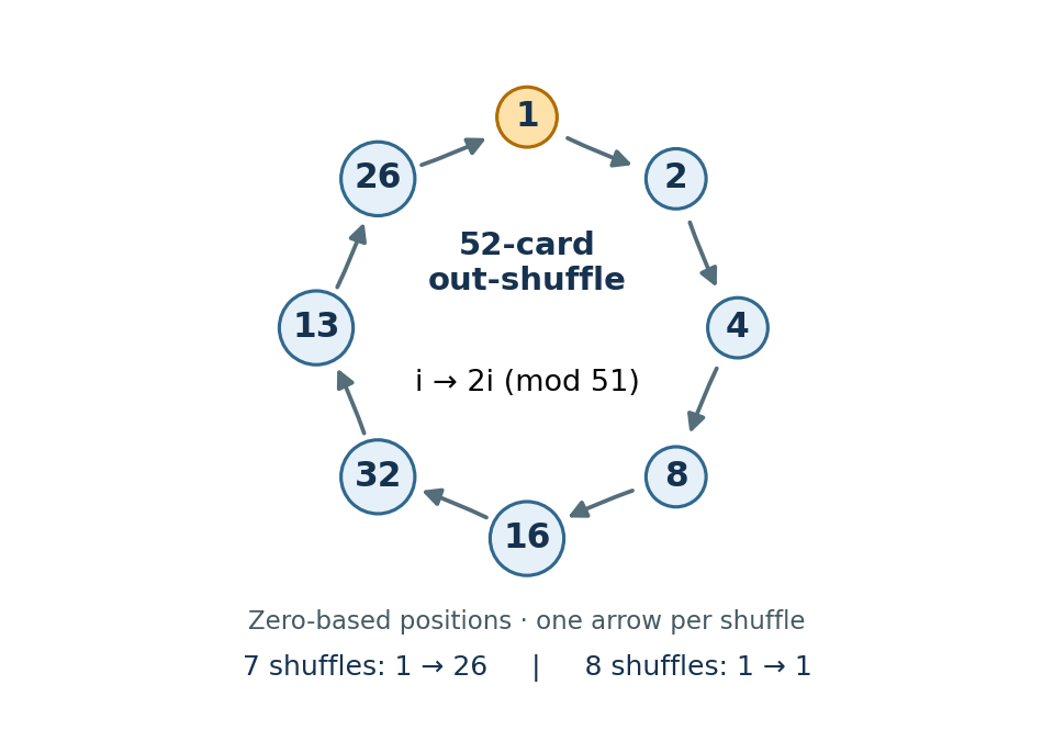
An eight-step position cycle under the 52-card perfect out-shuffle
. Details. 
This single position already disproves a seven-step return; the modular calculation proves that the whole permutation returns after eight.
Apply the supplied bitonic-merging fact directly:For length ,
merge :: Ord a => [a] -> [a]
merge xs = rounds (levels (length xs)) xs
  where
    levels n
      | n <= 1    = 0
      | otherwise = 1 + levels (n `div` 2)
    order (x,y)
      | x <= y    = (x,y)
      | otherwise = (y,x)
    pass = unpairs . map order . pairs . riffle
    rounds 0 ys = ys
rounds r ys = rounds (r-1) (pass ys)levels n = k. Each pass performs exactly the required shuffle and adjacent compare-exchange operations. The supplied fact therefore proves that rounds k yields ascending order from a bitonic sequence. Each pass preserves the multiset of entries and costs , giving time for . Length one needs no pass. The definition also harmlessly returns [] on empty input.Sort the two halves ascending, reverse the second, and concatenate to form a bitonic sequence:For a power-of-two length greater than one, both halves are smaller powers of two. By induction, the recursive calls return ascending permutations of their respective inputs. Reversal makes the second half descending, so part (e)'s precondition holds and
sort :: Ord a => [a] -> [a]
sort []  = []
sort [x] = [x]
sort xs  = merge (sort as ++ reverse (sort bs))
where (as,bs) = halve xsmerge sorts their concatenation without losing entries. This proves both sortedness and sorting permutation preservation. Its recurrence relation is , so summing the levels gives time. Equal keys cause no difficulty; ascending and descending here permit equality. This is a bitonic sorting algorithm.For the first recurrence relation, the master theorem compares with . Since , the recursive leaves dominate and the answer is . More explicitly, the work at depth is , a growing geometric series that stops at depth , where its sum has that order.
For the second recurrence relation, each step subtracts two and adds one until reaching a base case. For integral there are steps, so and the answer is .
The third set of printed requirements is inconsistent. The specified base values and its recurrence relation give identically, as strong induction immediately verifies: . In particular , while the extra condition demands . Thus no function satisfies all the printed conditions. Dropping that extra inequality gives .
The likely intended growth calculation can nevertheless be made precise, without treating it as a solution of the contradictory data. On dyadic arguments put . Its equation has the general formbecause has characteristic equation . The printed values force . With suitably different initial values, the condition for arbitrarily large instead requires , hence and , or . That last order describes corrected initial data, not the paper as printed. All three bullets belong to this single marked part.
Maintain the two largest entries of each segment, counting repeated values as separate entries. A singleton returns its value and a sentinel for its missing runner-up. Split a longer segment into two nonempty halves, recursively obtain and , and combine them byFor example, an implementation on an indexed sequence can use:The result is
top2(lo, hi):
    if hi-lo == 1: return (a[lo], -infinity)
    mid = (lo+hi)//2
    (mL,sL) = top2(lo,mid)
    (mR,sR) = top2(mid,hi)
    if mL >= mR: return (mL, max(sL,mR))
else: return (mR, max(mL,sR))top2(0,n). The global maximum is one of the two child maxima. Once its side is identified, the global second maximum is either that side's runner-up or the other side's maximum; the displayed formula exhausts these possibilities. This proves the divide-and-conquer algorithm by induction on segment length. There are leaves and constant-cost combinations, so its time complexity is , with recursive stack space for balanced splits. A Maybe value can replace the formal sentinel for a generic ordered element type. If both largest entries are equal, both are returned; a second distinct value is a different specification.For each segment retain its total weight , largest possibly-empty prefix weight , largest possibly-empty suffix weight , and largest possibly-empty internal contiguous weight . The maximum-subarray segment summary combines adjacent segments asAn empty segment has all four values zero. For a singleton of weight , use . The recursive procedure splits into halves, computes their summaries and applies these four formulas; the root's is the desired maximum weight.
To return an actual subsequence, attach half-open endpoints to each of . A prefix endpoint starts at its segment's left boundary, and a suffix endpoint ends at its right boundary, including empty prefixes and suffixes. Store the interval belonging to whichever candidate wins a maximum. The crossing candidate joins a left suffix to a right prefix, which meet at the split point; the other candidates keep their child endpoints. Choose an empty interval on ties at weight zero. Return the root's winning interval as a slice of the original input. This augmentation still has constant-size state and constant-time combinations.
For correctness, a prefix either stays inside the left half or consists of the entire left half and a right prefix. The suffix argument is symmetric. An optimal contiguous segment either lies in one half or crosses the split, in which case it consists of a left suffix and a right prefix. Each upper bound in the formulas is attained by its recorded candidate, proving exactness. Empty candidates ensure that an all-negative input returns the empty subsequence.
There are tree nodes, each using a constant number of additions and comparisons. The divide-and-conquer algorithm therefore takes time and stack space, plus the cost of copying the returned slice if a copy is required. In the stated example it selects zero-based interval of weight 8. Carrying all four summary values avoids rescanning the halves at each split.
Use positive integral item weights and a nonnegative integral capacity. For the unbounded knapsack problem, define to be the best value with total weight at most . ThenThe zero candidate is the empty selection, so unused capacity is allowed and an empty set of fitting items causes no problem. Every nonempty feasible selection has some last item ; removing one copy leaves a feasible solution at capacity . Its value is bounded by the corresponding candidate. Conversely, taking an optimal smaller selection and adding that item attains the candidate, proving the recurrence relation by optimal substructure. Positive weights make every dependency strictly smaller.
Fill capacities in increasing order. There are entries, each scanning items, so the dynamic programming takes time and storage. A winning item pointer at each capacity reconstructs the chosen multiplicities. These are capacity-dependent, pseudopolynomial bounds. For zero-weight items, any positive value makes the repetition problem unbounded; nonpositive-value zero-weight items may simply be discarded before using the recurrence.
Capacity alone cannot say which items have already been used. For the 0-1 knapsack problem, let use only the first items, each at most once. ThenThe two alternatives omit item or take it. In the latter case its remaining companions must solve the smaller problem using the first items; otherwise replacing them would improve the whole selection. Both branches reduce the item index, so taking item cannot take it again. This establishes the recurrence relation and optimal substructure.
Fill rows in increasing and return . There are entries with constant work each. Store the decisions for reconstruction; value-only computation uses space by keeping two rows, or by scanning capacities downwards in a single row. A forward scan in a single row would instead allow repetitions. Nonnegative integral weights suffice for this version, including zero-weight items, because the item index always decreases.
This version of Kadane's algorithm, named for Joseph Born Kadane, permits the empty subsequence. For , let be the maximum of zero and the weight of a contiguous subsequence ending exactly at position . Let be the best weight anywhere in the first positions. UseA segment ending at either extends one ending at or starts at ; the zero candidate permits discarding a negative predecessor and the empty answer. Any best segment of the first positions either ends at or already occurs in the first . These two decompositions prove the dynamic programming equations by induction.
Here is an implementation returning endpoints, using zero-based indexing:There is exactly one addition per input element, hence additions and comparisons. Auxiliary storage is . The all-negative case retains interval and weight zero. The example returns and weight 8, hence the desired contiguous subsequence.
best_segment(a):
    end_weight = best_weight = 0
    start = best_lo = best_hi = 0
    for j in range(len(a)):
        trial = end_weight + a[j]
        if trial <= 0:
            end_weight = 0
            start = j+1
        else:
            end_weight = trial
        if end_weight > best_weight:
            best_weight = end_weight
            best_lo, best_hi = start, j+1
return (best_lo, best_hi, best_weight)The Dijkstra algorithm finalises vertices in the order . After finalising , tentative distances to are . Finalising sets the distance to to . Finalising sets the distance to to . Finalising improves the distance to to ; its edge to proposes and causes no improvement. The final distance vector in vertex order is . All weights are positive, so every finalisation is justified by the usual label-setting shortest-path algorithm invariant. The method is named for Edsger W. Dijkstra.
The intermediate states of the Bellman-Ford algorithm depend on edge order. Specify in-place edge relaxation in lexicographic directed-edge order:Starting with , the first pass changes the vector as follows; omitted relaxations make no change:The next pass makes no change, allowing early termination. If all passes are performed, passes two through four retain .
For the synchronous convention, where every relaxation reads only the previous row, the Synchronous Bellman-Ford recurrence instead givesBoth conventions reach the same shortest distances. The algorithm's eponyms are Richard Bellman and L. R. Ford Jr..
Let and replace every edge weight by . Call the supplied shortest-path routine once using these new weights, and return its path in the original graph. For every path ,where is its number of edges. Positive original weights imply positive transformed weights, so a shortest route can be taken to be simple and has at most edges. Distinct integral original weights of paths differ by at least one. Thus if for simple paths, thenFor equal original weights, the transformed comparison is exactly the comparison of hop counts. Therefore every transformed shortest path minimises original weight first and number of edges second, proving the integer-weight shortest-path tie-breaking lemma. The transformation costs time, followed by one subroutine call. Weights gain only bits; exact arithmetic should be used if multiplying machine-sized weights might overflow. If is unreachable, it remains unreachable.
Use a dynamic programming state indexed by an edge budget. Put and for , then for computeEvery route using at most edges either already uses at most , or ends with some edge whose preceding route uses at most . Conversely every finite candidate in the displayed equation is attained by such a route. This proves the hop-bounded shortest-route recurrence by induction on , even when weights are negative.
In each round, copy the previous distance row and relax every edge into the new row, always reading from the old row. An in-place pass would allow several new edges in one round and violate the edge budget. Store a predecessor record for every selected candidate, either a carry to or the incoming edge from . Following records backwards from and reversing the collected edges returns the actual optimum route; an infinite final distance means no feasible route exists.
Only vertices incident to an edge, together with , need distance fields. In a graph representation whose edges reference vertex records, initialise those fields by visiting both endpoints of every edge, then ; repeated initialisations are harmless. In each round, first copy old fields to new fields by another complete endpoint pass, and only then begin the relaxation pass. Copying the same endpoint several times before any relaxation also does no harm. Thus each round costs , with no scan of isolated vertices, and for the total is time. An implementation that instead initialises full arrays for all vertices has the conventional bound . For or no edges, only the empty route can succeed.
To realise reconstruction without a dense table, associate a persistent route record with each finite distance. A successful relaxation in round creates a record containing the new edge and a pointer to the old round's route record at its source; a carry shares its record. All reads use old-round records. At most such records are created, taking space, and the returned chain has at most edges. Distances alone need only two fields per relevant vertex.
Here “route” uses the standard edge-budget shortest-path convention permitting repeated vertices; a bounded budget prevents an arbitrarily long negative-cycle traversal. If “path” instead requires vertex simplicity with unrestricted negative weights, this recurrence does not enforce that extra restriction. With nonnegative weights, removing cycles gives a simple optimum within the same budget.
Start Prim's algorithm at vertex , since the source does not specify a starting vertex. Write every undirected edge with its smaller endpoint first. With lexicographic tie-breaking, the accepted edges are , of total weight 9.
Initially is the cheapest crossing edge. The next minimum is a weight-two tie between and , so choose . Then the weight-two tie between and is resolved in favour of . Adding vertex exposes the weight-one edge , which is selected next. Finally precedes among the weight-three choices. Every accepted edge crosses from the existing tree to a new vertex, as required by the minimum spanning tree cut property. A different starting vertex can produce a different accepted-edge order; the displayed answer fixes that unspecified choice. The algorithm is named for Robert C. Prim.
Sort edges by weight and then lexicographically. Kruskal's algorithm accepts , again of total weight 9.
The two weight-one edges join different components. Among weight-two edges, is accepted, then joins the two larger components; would now create a cycle and is rejected. Among weight-three edges, is rejected for the same reason, and joins the remaining vertex. Five accepted edges connect all six vertices, so the algorithm can stop. The disjoint-set data structure implements precisely these component tests. The eponym is Joseph Kruskal.
To find a minimum-weight acyclic subgraph, filter to the subgraph containing only strictly negative-weight edges, and run Kruskal's algorithm on those edges, accepting an edge exactly when it joins different current components. Return the resulting forest, with any omitted vertices regarded as isolated. Zero-weight edges may be omitted without worsening the objective.
To prove correctness, first remove all nonnegative edges from any feasible acyclic graph; removing them preserves acyclicity and cannot increase weight. Thus an optimum using only negative edges exists. Inside a connected component of , any forest not yet connected can be extended by a negative crossing edge: some such edge exists because the original component is connected. Adding it preserves acyclicity and strictly reduces total weight. Consequently an optimum must span each component of , and its restriction there must be a minimum spanning tree. Kruskal's algorithm finds exactly the resulting minimum spanning forest of . This proves optimality among all acyclic subgraphs, including disconnected ones.
With negative edges, filtering costs , sorting costs , and the union-find operations take time. A standard overall bound is time. If there are no negative edges, the empty edge set is optimal.
Assume the graph is connected so that a minimum spanning tree exists, and let be the output of Kruskal's algorithm. With distinct weights there is a strict total edge ordering. Suppose another minimum spanning tree existed. Choose and increase only by a positive so small that the strict ordering of all edge weights remains unchanged. For a finite graph such an exists, using less than the gap to the next larger weight; if is largest, any sufficiently small positive increase works.
Running Kruskal's algorithm again examines exactly the same order and makes exactly the same component decisions. It therefore still returns , which must remain optimal for the perturbed weights. But has become more expensive by , while is unchanged. They had equal original weight, so now is cheaper, a contradiction. This proves that distinct weights imply a unique minimum spanning tree.
The converse is false. A triangle with edge weights has a unique minimum spanning tree, consisting of its two weight-one edges. Its total is , while either other spanning tree has total . Thus equal edge weights permit, but do not force, multiple optimum trees. The same perturbation proof applies componentwise to a minimum spanning forest.
Articles by others on the same topic
There are currently no matching articles.