Trinity Term 2023, 13 June, 14:30–17:30. Three-hour Year 1 of the computer science course of the University of Oxford paper.
Public source archive. The paper is archive member
2022/T/a10097w1.pdf; its cover identifies the sitting as 2023.A strict function satisfies , where is the bottom value representing an undefined or nonterminating computation. This is a semantic implication: obtaining a defined result requires enough definedness of the argument. It does not prescribe an evaluation order or say that every component of a structured argument is evaluated.[ref]
For example, in Haskell,is strict, since every result is , but never needs to inspect its argument. Moreover, lazy evaluation may leave an entire application unevaluated when its result is unused. Strictness is therefore different from the operational statement that an argument is evaluated on every call.
f :: a -> b
f _ = undefinedThe list fold criterion is: there must be a value
z and a definable combining function c such thatThe last equality says that all information needed about the tail factors through f xs; the combining function receives no other access to xs. These conditions give f = foldr c z.Necessity follows from the defining equations of
foldr, including its case distinction on the input list. Sufficiency follows by structural induction for finite lists and finite partial-list approximations. For infinite or partial lazy lists, the usual continuous semantics of these definable functions extends equality from the approximations to their limit. The strictness condition matters: agreement only on finite total lists does not establish agreement at . This is the fold factorisation criterion.Use these structural recursion definitions in Haskell:The first definition returns a known outer constructor even when
tails :: [a] -> [[a]]
tails xs = xs : ptails xs

ptails :: [a] -> [[a]]
ptails [] = []
ptails (_:xs) = tails xs

ntails :: [a] -> [[a]]
ntails [] = []
ntails xs@(_:rest) = xs : ntails restxs is undefined, so null (tails undefined) is False, as required. The pattern in ntails must first determine whether the input is empty. Each suffix of a list is shared with the original list; on a finite input of length , constructing the outer lists takes work and additional outer-list space. No suffix is copied or measured repeatedly.tails is not a direct list fold. Every foldr c z is strict in its list argument, but tails undefined = undefined : undefined has a defined outer constructor. Applying null distinguishes this result from .ptails is not a direct list fold either. On a type with distinct values u and v,A fold step given the same new head x and these equal folded tails must return the same result. However,Thus the tail information needed by the next step does not factor through ptails; this violates the fold factorisation criterion even on finite total lists.ntails is a direct list fold:ntailsFold :: [a] -> [[a]]
ntailsFold = foldr step []
where
step x yss = (x : original yss) : yss
original [] = []
original (ys:_) = ys[]. Hence original (ntailsFold xs) = xs. The inner case distinction is delayed beneath constructors, so the definition also preserves the required behaviour on partial and infinite lazy lists. Building a suffix head does not first demand the whole folded tail.For prefixes of a list, the corresponding Haskell definitions areThe empty prefix is available without inspecting the input in
inits :: [a] -> [[a]]
inits xs = [] : ninits xs

pinits :: [a] -> [[a]]
pinits [] = []
pinits (x:xs) = [] : map (x:) (pinits xs)

ninits :: [a] -> [[a]]
ninits [] = []
ninits (x:xs) = map (x:) (inits xs)inits. Every nonempty prefix of a list begins with its input's head, explaining the last equation. For pinits (x:xs), prepend x only to proper prefixes of xs, and include the empty prefix.On finite inputs,
inits [] = [[]], whereas both other functions return []. On an infinite input, all finite prefixes are proper and these definitions produce them incrementally. Fully constructing all elements of all prefixes takes work for an input of length , matching the size of that output; there are no repeated end-append operations to add another factor.inits is not a direct list fold: inits undefined = [] : undefined has a defined outer constructor, while foldr c z undefined is .Both For
pinits and ninits are direct list folds:pinitsFold :: [a] -> [[a]]
pinitsFold = foldr (\x yss -> [] : map (x:) yss) []
ninitsFold :: [a] -> [[a]]
ninitsFold = foldr (\x yss -> [x] : map (x:) yss) []pinits, the combining function is exactly the recursive step above. For ninits, expand inits xs = [] : ninits xs and useNeither step needs to inspect yss before producing its first outer constructor. Thus the definitions satisfy the fold factorisation criterion on partial as well as total lazy lists.Use arbitrary-precision integers for positions, avoiding overflow on infinite sequences:The type synonym
type Seq a = a -> [Integer]

rep :: Eq a => [a] -> Seq a
rep xs v = [i | (i,x) <- zip [0..] xs, x == v]Seq a needs no equality constraint; the equality test is required specifically by rep. The list comprehension visits input positions in increasing order, so the output is an increasing list of precisely the matching positions. For finite inputs this includes a terminating empty list when the value is absent. Infinite inputs require the additional productivity distinctions discussed below. This is an occurrence-position representation of a sequence.With nonpositive counts treated as in the standard list operations:An occurrence survives
takeSeq :: Integer -> Seq a -> Seq a
takeSeq n s
  | n <= 0 = const []
  | otherwise = \v -> takeWhile (< n) (s v)

dropSeq :: Integer -> Seq a -> Seq a
dropSeq n s
  | n <= 0 = s
| otherwise = \v -> map (subtract n) (dropWhile (< n) (s v))takeSeq n exactly when its original index is less than , and its index stays unchanged. It survives dropSeq n exactly when its original index is at least , and its new index is the original one minus . Sorted occurrence lists justify takeWhile and dropWhile. No equality constraint on the element type is needed because the operations only transform positions. The first guard also lets takeSeq 0 s v return [] without inspecting s v.The most informative occurrence-position representation of a sequence of natural numbers isEach nonnegative integer occurs once at its own index, and negative integers never occur.
naturals :: Seq Integer
naturals v
  | v < 0 = []
| otherwise = [v]This is not equal to
rep [0..] under lazy evaluation. For a nonnegative query v, rep eventually emits v, but then searches forever for another occurrence: its result has the shape v : undefined, rather than the terminating singleton [v]. For a negative query, even the outer constructor is never produced, whereas naturals immediately returns [].No general, correct
rep :: Eq a => [a] -> Seq a can always certify those absences from an arbitrary infinite input. A terminating certification has inspected only finitely many elements, and the same prefix could be followed by the supposedly absent value, or by a further occurrence of it. Extra knowledge changes the problem: for a promised strictly increasing integer input, a search can stop with [] when it first exceeds the query and return [i] immediately upon equality. That specialised representation can produce naturals; a generic search cannot. This is the absence-detection obstruction for infinite lists.Even and odd original positions become consecutive new positions:An occurrence at belongs to
evens :: Seq a -> Seq a
evens s v = map (`div` 2) (filter even (s v))

odds :: Seq a -> Seq a
odds s v = map (`div` 2) (filter odd (s v))evens at position ; one at belongs to odds at position . Thus the formulas preserve increasing position order and produce the specified finite examples. For infinite occurrence lists, filtering can search forever when no further position of the chosen parity exists. Consequently these otherwise direct formulas need not preserve productivity for every query.Define the ordered merge algorithm explicitly:The first sequence occupies even positions and the second occupies odd positions. Within each transformed list, order is preserved; merging puts all positions for a queried token into increasing order. The two transformed lists have disjoint parities, so equality cannot occur between their heads on valid inputs. The length assumption ensures that these positions describe the intended interleaved sequence without a gap at its finite end.
mergePos :: [Integer] -> [Integer] -> [Integer]
mergePos [] ys = ys
mergePos xs [] = xs
mergePos xs@(x:xt) ys@(y:yt)
  | x <= y = x : mergePos xt ys
  | otherwise = y : mergePos xs yt

ilv :: Seq a -> Seq a -> Seq a
ilv s t v = mergePos (map (2*) (s v))
(map (\j -> 2*j+1) (t v))For finite, fully defined representations, yes; for arbitrary infinite ones in Haskell, no. At the level of mathematical occurrence sets, splitting by parity, dividing by two, and then applying the inverse index transformations recovers every original position exactly once. Thus the equality holds on finite total position lists.
For a proper infinite representation, take the alternating Boolean sequence, represented byThis is a total representation: both queries return productive infinite occurrence lists. Butfilters for odd indices in uses
alternating :: Seq Bool
alternating False = [0,2..]
alternating True = [1,3..]odds alternating False[0,2..], so it produces no outer constructor and denotes . The callilv (evens alternating) (odds alternating) FalsemergePos to inspect both transformed lists before emitting its first result; it therefore also diverges. In contrast, alternating False starts with 0. Applying head distinguishes the two. The productivity failure is real even though the mathematical position-set identity is correct; the hypothesis that the input properly represents an infinite sequence does not remove it.First remove a single matching token, so duplicates cannot be reused:Equal game lengths are assumed. For each token,
pluck :: Eq a => a -> [a] -> Maybe [a]
pluck _ [] = Nothing
pluck x (y:ys)
  | x == y = Just ys
  | otherwise = case pluck x ys of
      Nothing -> Nothing
      Just zs -> Just (y:zs)

overlap :: Eq a => [a] -> [a] -> [a]
overlap [] _ = []
overlap (x:xs) ys = case pluck x ys of
  Nothing -> overlap xs ys
  Just zs -> x : overlap xs zs

scoreBC :: Eq a => [a] -> [a] -> (Int,Int)
scoreBC secret guess = (bulls, matches - bulls)
  where
    bulls = length [() | (s,g) <- zip secret guess, s == g]
matches = length (overlap guess secret)overlap retains exactly the smaller of its two multiplicities, so its length is the multiset overlap. It never spends a secret occurrence twice. Positional matches account for bulls; after reserving them, each token's remaining possible matches decrease by exactly its bull count. Hence matches - bulls counts precisely the cows. The source example gives (1,1). With equality as the only operation on tokens, these definitions take time for length .Use a distinct constructor for each mark, and reserve every bull before allocating any cow:The multiset
data Mark = Bull | Cow | Miss deriving (Eq,Show)

scoreWordle :: Eq a => [a] -> [a] -> [Mark]
scoreWordle secret guess = mark pairs pool
  where
    pairs = zip secret guess
    pool = [s | (s,g) <- pairs, s /= g]
    mark [] _ = []
    mark ((s,g):ps) available
      | s == g = Bull : mark ps available
      | otherwise = case pluck g available of
          Nothing -> Miss : mark ps available
Just rest -> Cow : mark ps restpool contains exactly the unused secret tokens after all bulls have been set aside. The recursive invariant is that available contains those tokens not yet allocated to cows. A successful pluck consumes one, and failure leaves the pool unchanged. This proves both multiplicity correctness and the priority of bulls over cows. Among duplicate non-bull guess tokens, the leftmost eligible ones receive cows. For secret "alpha" and guess "aaabb", the result is [Bull,Cow,Miss,Miss,Miss]. This implements duplicate-aware positional scoring.A scorer applies the same scoring rule, with the fixed secret, independently to each guess:The first score depends only on the first guess, and every later score only on the corresponding guess. Thus this player has no unguarded dependence on its own future output when connected to the guesser by a lazy feedback stream. Neither the dictionary nor a strategy is needed by a truthful scorer once the secret and scoring rule are fixed.
mkScorer :: (secret -> guess -> score)
         -> secret -> [guess] -> [score]
mkScorer score secret = map (score secret)
The score function takes a proposed secret first and a guess second:Assume that the initial dictionary contains the secret, that scores are truthful, and that
mkGuesser :: Eq score
          => (guess -> guess -> score)
          -> ([guess] -> guess)
          -> [guess] -> [score] -> [guess]
mkGuesser score strategy dictionary = play dictionary
  where
    play candidates replies =
      let g = strategy candidates
      in g : case replies of
          [] -> []
r:rs -> play [s | s <- candidates, score s g == r] rsstrategy returns a candidate from its nonempty input. The candidate invariant is exactly the dictionary entries consistent with every score already received. Filtering by score s g == r establishes the same invariant after the next reply and retains the true secret.Crucially, the next guess
g is placed under the outer list constructor before replies is inspected. It depends on earlier replies only; the first guess depends on none. This guarded lazy feedback stream makes the mutually recursive game productive whenever the strategy and scoring operations terminate. Moving the case replies outside the constructor would create a circular demand before the first guess.Let be the number of distinct dictionary candidates. A wrong guess is itself a current candidate, but its actual score differs from its score against itself, which has all positions as bulls. Therefore each wrong reply removes at least that candidate while retaining the true secret. There can be at most wrong guesses. A correct guess leaves only the secret consistent with the all-bull reply. Hence every such infinite game's history eventually has the constant tailThis is the finite candidate elimination bound; it assumes a nonempty finite dictionary of fixed-length secrets and a strategy that chooses from the remaining candidates.
The stated end condition is identification, so stop when just one candidate remains, even if it has not been guessed. Replace the worker above byThe scorer can stay
play [] _ = []
play [_] _ = []
play candidates replies =
  let g = strategy candidates
  in g : case replies of
      [] -> []
r:rs -> play [s | s <- candidates, score s g == r] rsmap (score secret): once the guess list ends, its score list ends too. The unchanged game then returns a finite history, with at most rounds; a singleton initial dictionary needs no round. If the identified secret is also wanted as an explicit output, return that sole surviving candidate alongside the history.Use the source's constructor order: left subtree, root value, right subtree.A tree fold replaces the two constructors by an algebra on already folded children. A tree unfold expands a seed either into the empty tree or into a root value and two new seeds. The definitions themselves work on arbitrary binary trees; preserving the binary search tree ordering requires the supplied algebra or seed expansion to respect its bounds.
data Tree a = Tree (Tree a) a (Tree a) | Empty

foldTree :: (b -> a -> b -> b) -> b -> Tree a -> b
foldTree node empty Empty = empty
foldTree node empty (Tree l x r) =
  node (foldTree node empty l) x (foldTree node empty r)

unfoldTree :: (s -> Maybe (s,a,s)) -> s -> Tree a
unfoldTree next seed = case next seed of
  Nothing -> Empty
  Just (ls,x,rs) ->
Tree (unfoldTree next ls) x (unfoldTree next rs)The direct tree fold for an inorder traversal isBy structural induction, the child lists are ascending; the binary search tree property places every left value below the root and every right value above it. The displayed list concatenation therefore gives an ascending list containing every stored value exactly once.
flattenFold :: Tree a -> [a]
flattenFold = foldTree (\ls x rs -> ls ++ (x:rs)) []For a version with linear time complexity on every tree shape, use an accumulator:This also has a higher-order tree fold expression using difference lists:Its folded value is a function that prepends the inorder traversal to a supplied tail. The accumulator invariant is
flatten :: Tree a -> [a]
flatten t = onto t []
  where
    onto Empty zs = zs
onto (Tree l x r) zs = onto l (x : onto r zs)flattenLinear :: Tree a -> [a]
flattenLinear t =
foldTree (\l x r -> l . (x:) . r) id t []onto t zs = flattenFold t ++ zs. Each node contributes one constructor, giving time to consume the output. By contrast, the direct list-valued fold can take on a left-skewed tree because ++ repeatedly copies left traversals.Choose the middle element as the root:The input is a finite, strictly ascending list, as required for distinct elements of a set. The two child lengths differ by at most one. Applying the same argument recursively gives a balanced binary tree of logarithmic height. All values on each side retain their original order, proving the binary search tree property. With linked lists, the repeated splitting gives time; it does not repeatedly insert values into a skewed tree.
build :: [a] -> Tree a
build [] = Empty
build xs = Tree (build ls) x (build rs)
  where
(ls,x:rs) = splitAt (length xs `div` 2) xsUse the remaining ascending list itself as the seed:The empty seed produces
buildUnfold :: [a] -> Tree a
buildUnfold = unfoldTree split
  where
    split [] = Nothing
    split xs =
      let (ls,x:rs) = splitAt (length xs `div` 2) xs
in Just (ls,x,rs)Empty. Every nonempty seed produces exactly the midpoint and two child seeds used by build. Thus the defining equations agree, and structural induction on the finite input proves buildUnfold xs = build xs. The balance and ordering arguments carry over unchanged.Fold into a membership predicate:At an empty tree the predicate is always false. At a nonempty binary search tree, an unequal query can occur only in the indicated child, while equality finds the root. This proves correctness inductively. Under lazy evaluation, the unused folded child is not demanded; lookup follows one root-to-leaf route and takes comparisons in a tree of height . Defining the predicate by a fold does not require visiting both subtrees for each query.
find :: Ord a => Tree a -> a -> Bool
find = foldTree node (const False)
  where
    node left x right q = case compare q x of
      LT -> left q
      EQ -> True
GT -> right qInsert down the unique search route, leaving equal elements unchanged:The binary search tree ordering determines the only child in which a missing query can belong. The recursive call preserves that child's ordering bounds, and the other child is shared. Thus the output represents the original set with
insert :: Ord a => a -> Tree a -> Tree a
insert q Empty = Tree Empty q Empty
insert q t@(Tree l x r) = case compare q x of
  LT -> Tree (insert q l) x r
  EQ -> t
GT -> Tree l x (insert q r)q added, with duplicates suppressed. Its time complexity and newly allocated route length are ; it makes no balancing guarantee.A tree fold can compute insertion while retaining the unchanged children by carrying a pair. The following fold-derived implementation preserves the lazy evaluation behaviour of part (f):The invariant of the folded pair is
insertViaFold :: Ord a => a -> Tree a -> Tree a
insertViaFold q t = snd (foldTree node base t)
  where
    base = (Empty, Tree Empty q Empty)
    node ~(l,li) x ~(r,ri) = (original,updated)
      where
        original = Tree l x r
        updated = case compare q x of
          LT -> Tree li x r
          EQ -> original
GT -> Tree l x ri(original subtree, subtree with q inserted). The empty case establishes it. At a node, the first components reconstruct the original tree, and the second components supply whichever child insertion is needed. The irrefutable pair patterns ~(l,li) and ~(r,ri) avoid demanding an unused child's fold. Induction on finite approximations therefore proves equivalence even for partial trees, and only the selected search route needs insertion work.There is a distinction if “written as a fold” is required to mean a direct same-result-type expression Here
insert q = foldTree node base, with no richer result and final projection. On finite fully defined binary search trees, such an expression is possible by undoing insertion of a new extreme key in the child that should remain unchanged. For completeness, a literal direct fold on that finite, fully defined domain is:eraseFresh :: Ord a => a -> Tree a -> Tree a
eraseFresh _ Empty = Empty
eraseFresh q (Tree l x r) = case compare q x of
LT -> Tree (eraseFresh q l) x r
EQ -> Empty
GT -> Tree l x (eraseFresh q r)
insertDirectFold :: Ord a => a -> Tree a -> Tree a
insertDirectFold q = foldTree node (Tree Empty q Empty)
where
node left x right = case compare q x of
LT -> Tree left x (eraseFresh q right)
EQ -> Tree (eraseFresh q left) x (eraseFresh q right)
GT -> Tree (eraseFresh q left) x righteraseFresh is used only to undo a newly inserted extreme key, which is a leaf; it is not a general deletion operation. The binary search tree bound at each root guarantees exactly that precondition on every child being restored.On all partial Haskell trees, however, a direct expression with result type
Tree a cannot implement part (f).For that obstruction, fix Both can be completed to valid right subtrees of a root labelled
q = 0, and consider the two right subtreesr1 = Tree Empty undefined Empty
r2 = Tree Empty undefined (Tree Empty 3 Empty)1. Yet insert 0 r1 and insert 0 r2 are both bottom, because insertion must compare 0 with their undefined root label. A direct fold equal to insertion would therefore receive the same folded left value, root 1, and bottom folded right value on both larger trees Tree Empty 1 r1 and Tree Empty 1 r2. It must return the same result. Part (f) instead preserves r1 or r2, which are distinguishable by inspecting their right-child constructors without inspecting the undefined labels. This proves the direct-fold obstruction. The pair-valued implementation avoids losing that information and states precisely which sense of fold implementation is being used.Start with . With in-place edge relaxation, the Bellman-Ford algorithm makes the following changes during its first lexicographic pass:The next pass makes no change; any remaining fixed-count passes also make none. Thus the final vector is . These are sequential updates within a pass, rather than the simultaneous values of the Synchronous Bellman-Ford recurrence.
Use source , as in the preceding part. The Dijkstra algorithm extracts vertices in the order . Distances after relaxing the outgoing edges of each extracted vertex areThe shortest path to is , with weight ; the direct route to and the route via are both heavier.
Take the directed graph with source and weighted edgesIt is a Directed acyclic graph, so has no negative-weight graph cycle. The true shortest path to is , of weight .
The standard label-setting shortest-path algorithm version of the Dijkstra algorithm extracts , then at distance , then at distance , and only then at distance . Thus it finalises instead of . Even if an implementation subsequently changes the stored label of the already settled vertex , it does not reprocess its outgoing edge to , so the error at remains. Allowing repeated reprocessing would instead be a label-correcting shortest-path algorithm, not the usual Dijkstra guarantee.
First run breadth-first search, ignoring weights, to obtain the minimum number of edges from the source to each reachable vertex. Then compute weighted distances only along edges that advance one breadth-first layer:Unreachable vertices keep distance . For an undirected graph, scan both orientations of each edge.
d[source] = 0; all other d[v] = infinity
for u in nondecreasing BFS-layer order:
    for each outgoing edge (u,v):
        if h[v] == h[u]+1:
            if d[u]+w(u,v) < d[v]:
                d[v] = d[u]+w(u,v)
predecessor[v] = uTo justify discarding other routes, a shortest path can be taken simple because every weight is positive. A simple path of edges has weight inEvery path with at least edges weighs at least . Consequently every minimum-weight path must also have the minimum possible number of edges: this is minimum-hop dominance for nearly unit weights.
A minimum-hop path to uses exactly edges. Every prefix of such a path must itself have minimum hop count, since replacing a longer prefix by a shorter one would shorten the whole route. Hence it advances from layer to layer at every step. The retained edges form a Directed acyclic graph, ordered by . The displayed dynamic programming recurrence therefore finds the cheapest of all minimum-hop paths, which by the preceding bound is a true shortest path.
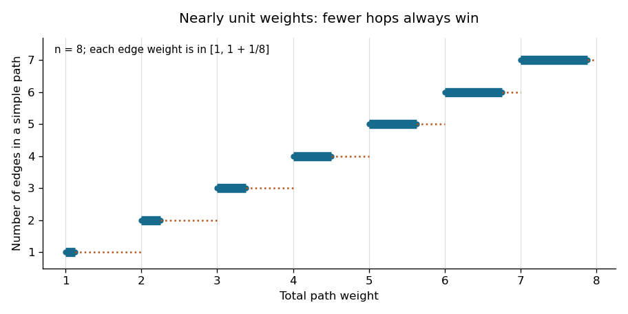

With an adjacency list, both the breadth-first search and the layer-ordered relaxations take time and total storage, where . The queue order from breadth-first search already supplies the layer order; no sorting or priority queue is needed. This improves the usual binary-heap Dijkstra bound and is linear in the input size.
Increment a single clock on each discovery and finish, starting with clock zero. Lexicographic depth-first search givesThe first search tree has discovery edges , , . The edge returns to an active ancestor. Once that tree finishes, vertex is a new root whose neighbour is already finished, and vertex is the final root. This accounts for all twelve events in the DFS discovery and finishing times.
The only possibilities are . Vertex reaches all of . In depth-first search, all vertices reachable from an active vertex must have been discovered and finished before its own finishing event, except for active ancestors. None of these four can be an ancestor of , because none can reach . Thus all four are finished before finishes.
Vertex cannot already be finished at that point: its outgoing edge to would have caused to be visited before it could finish. It also cannot be a descendant of , since cannot reach . Therefore is either still undiscovered or an active ancestor. In the first case the only remaining events are discovery and finishing of , giving . In the second case the only remaining event is finishing of , giving .
Both occur. Starting the outer traversal with leaves undiscovered and gives time . Starting with and taking its edge to first makes an ancestor and gives time . The argument does not assume any particular order on the other edges.
The strongly connected components areThe directed cycle makes its three vertices mutually reachable. Vertex has no outgoing edge. Vertex reaches that cycle but has no return path from it, and vertex reaches the other components but has no incoming path from them. These facts exclude every further merger.
Sort the open intervals by increasing left endpoint. Scan them in that order, maintaining the largest right endpoint among previously seen intervals. For the next interval , report an intersection if ; otherwise set and continue. Equality is allowed: and do not meet because the intervals are open. For zero or one interval, return that they are mutually non-intersecting.
If , a previous interval with right endpoint has left endpoint at most and has positive length. Together with , this guarantees an interior common point. Conversely, if , every earlier interval ends at or before , so none intersects the new one. This loop invariant proves correctness. A comparison sort costs time and the scan costs .
For the lower bound, transform an input of integers for the element distinctness problem intoEqual integers produce identical, intersecting intervals. Unequal integers differ by at least one, so their intervals are disjoint. The answer therefore decides whether all the integers are distinct. Moreover, comparing any two constructed endpoints can be simulated by comparing their original integers and, only on equality, their fixed offsets or . Thus the transformation preserves the comparison model, rather than gaining extra information from arithmetic on arbitrary endpoints. The supplied distinctness lower bound gives comparisons, matching the upper bound. This is the comparison lower bound for interval disjointness.
Let , , and let be the minimum number of words chosen from , in their given order, whose concatenation equals the length- prefix of a list of . Use for impossibility. The boundary values areFor ,Here denotes indices . The first case omits . In the second, the last selected word is , so removing it leaves a solution using only earlier words for the shorter prefix. These are exhaustive alternatives. Conversely either alternative constructs a valid solution, proving the dynamic programming recurrence. Even an empty word causes no cycle because both alternatives use row .
Fill rows in increasing and store the chosen alternative for every finite entry. If , report no solution. Otherwise trace back from : a skip moves to ; a take records index and moves to . Reverse the recorded indices to obtain the required subsequence. Ties may choose either valid predecessor.
There are states. A substring comparison costs , so under the given bounds and the running time is , with storage including reconstruction choices. Two rows give working storage if only the optimum count is needed. For the source example, the optimum is three words, indices , whose concatenation is
010111. This is ordered word concatenation dynamic programming.The minimum spanning tree cut property says: if a cut of a graph respects an edge set contained in some minimum spanning tree, a minimum-weight edge across that cut is safe to add to , meaning that some minimum spanning tree contains together with that edge. Respecting means no edge of crosses the cut. In particular, any lightest cut edge belongs to some minimum spanning tree; a uniquely lightest cut edge belongs to every minimum spanning tree.
For the exchange argument, take a minimum spanning tree containing . If it lacks the chosen edge , add to create its fundamental cycle. The remaining route between 's endpoints crosses the cut at some edge , with . Since the cut respects , . Replacing by preserves a spanning tree, retains , and cannot increase weight. Hence it is also minimum. Strict inequality would contradict minimality, which gives the unique-lightest assertion.
For an illustration, take a triangle with weights , , . Across the cut , is the unique lightest edge and must be in every minimum spanning tree. The minimum tree is , of weight . With tied light edges, the existence assertion need not mean that every minimum spanning tree contains the particular tied edge chosen.
Write each undirected edge with its smaller endpoint first. Kruskal's algorithm orders candidates first by weight and then lexicographically:Thus the requested addition order isand the minimum spanning tree has total weight . Five accepted edges connect all six vertices, so the remaining weight-four edges need not be scanned.
TakeIts longest strictly increasing subsequences have length two. A subsequence starting with can continue with or with , but cannot use both in increasing order; one starting at has only after it.
The specified greedy algorithm may choose the longest increasing subsequence . The remaining sequence is , which needs two singleton increasing subsequences. The algorithm then uses three subsequences in total.
However, and partition the original sequence into two increasing subsequences. One is impossible because the original sequence is not increasing. Hence two is optimal and the greedy choice is suboptimal. This establishes the counterexample to removing a longest increasing subsequence without relying on a tie-breaking rule: the problem asks for a longest choice that can fail.
Repeatedly remove vertices whose current degree is less than . Implement the deletions with an adjacency list, a queue and a degree counter for each active vertex:The requested subgraph is understood to be nonempty; otherwise an empty output would make the degree requirement vacuous or undefined. For , any nonempty input graph already qualifies.
active[v] = True for every v
count[v] = degree(v)
queue all v with count[v] < k
while the queue is nonempty:
    remove v from the queue
    if not active[v]: continue
    active[v] = False
    for each neighbour u of v:
        if active[u]:
            count[u] -= 1
            if count[u] == k-1: queue u
return the subgraph induced by the active vertices,
       or report failure if there is no active vertex
The correctness invariant is that every subgraph with minimum degree at least has all its vertices still active. Initially this is immediate. When is deleted, its degree in the whole active induced subgraph is less than . Any candidate subgraph on active vertices has at most that many incident edges at , so cannot contain it. Thus the invariant survives every deletion.
At termination, every active vertex has current degree at least , since every counter initially below the threshold or subsequently crossing it was queued. A nonempty surviving induced subgraph is therefore a valid answer. If none survives, the invariant rules out every possible answer, including ones omitting additional edges. The result is the k-core, with the k-core peeling invariant proving that deletion order cannot destroy a valid solution.
Each vertex is enqueued at most once when initially deficient or first crossing the threshold. Each adjacency list is scanned once when its vertex is deleted. The running time is , and storage is including the input graph.
The three answers, in source order, are:
- . In the Master theorem, , , and grows polynomially faster than . The regularity condition holds because . For powers of three, expansion even gives .
- , and hence . The telescoping sum is .
- . Set and . Then , with constant base cost for . The Master theorem with , applies because is polynomially smaller than . Finally .
The change of variable in the third case handles the additive shift in the recursive argument exactly; it is not an unjustified deletion of the
+1. These Big theta notation conclusions use the usual admissible input sizes, or bounded integer rounding of subproblem sizes., approximately , arithmetic operations. Strassen's algorithm replaces an matrix multiplication by seven products of half-size blocks and a constant number of block additions and subtractions. ConsequentlyThe Master theorem applies with , , since . Padding an arbitrary matrix dimension to the next power of two changes the dimension by less than a factor of two and preserves this asymptotic bound. The cost model counts scalar arithmetic as constant time; it is not a bit-complexity claim for arbitrarily large integer entries.
Let . After each linear-time selection algorithm and partition, exactly elements are removed, so the successive input sizes are . Thus the standard efficient implementation takesHere selection can use median of medians for worst-case linear time; a suitable randomised linear-time selection routine gives the same bound in expectation. Merely sorting each remaining array would introduce an avoidable logarithmic factor.
Recursively partition into equal halves by rank, keeping the selected median in the lower half:All elements are distinct, so both halves have exactly elements. Since remains a power of two, every internal split occurs at a rank divisible by .
quantiles(A,k):
    if length(A) == k:
        return [maximum(A)]
    p = select the (length(A)/2)-th smallest element of A
    L = all elements of A at most p
    R = all elements of A greater than p
return quantiles(L,k) followed by quantiles(R,k)For correctness, the desired ranks in the lower half are . In the upper half they are the same local multiples of , shifted by . These are exactly all desired global ranks. At a leaf of size , its maximum is its sole requested local rank. Induction therefore proves that the output contains every requested order statistic, in increasing order, including the original maximum. There is no separate internal-node output of
p, which would duplicate a rank already supplied by the lower subtree.Use a worst-case linear-time selection algorithm and linear partitioning. The divide-and-conquer algorithm hasThere are internal levels, each with total work , and leaves with total work . Since the source assumes , the running time isThis is multiselection by balanced rank partitioning. In-place selection and partitioning can use the original array; the output has values. The multiselection recursion has depth ; the selection routine contributes its own auxiliary storage.
Articles by others on the same topic
There are currently no matching articles.