Let be an open set, , and a continuous function. Through every there is a local solution of a differential equation: a continuously differentiable function on an open interval containing , satisfying the displayed initial value problem pointwise. No Lipschitz condition is assumed.[ref]
Ordinary Differential Equations and Dynamical Systems by Gerald Teschl. Gerald Teschl, Ordinary Differential Equations and Dynamical Systems, §2.7, Theorem 2.19, printed p. 56: forward existence and the analogous backward result
Continuity of a proposed rate law therefore guarantees at least one trajectory for a short time. For a physical model, this is a first consistency check: can the stated rule and initial condition actually be followed? Prediction also needs uniqueness. The delayed solutions of a square-root differential equation below show how the same rule and initial condition can leave a departure time undetermined. The Picard-Lindelöf theorem supplies a sufficient additional hypothesis for uniqueness; failure of that hypothesis alone does not prove nonuniqueness.
For the initial value problem , , a forward solution of a differential equation can stay zero until any , then follow . The delayed solutions of a square-root differential equation verify this freedom exactly.
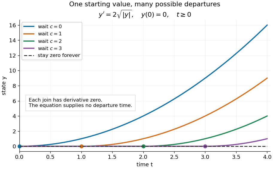
One initial condition admits an arbitrary forward waiting time
. Colored curves leave zero at the marked waits ; the dashed curve stays zero forever. Every curve satisfies the same original differential equation for . Details.Local existence gives neither a global solution of a differential equation nor a bound on all future values. The continuous function already permits finite-time blowup; the finite-dimensional continuation criterion explains the additional issue of extending a trajectory within its domain.
Proof outline: choose a compact set . By the extreme value theorem, . Take with . Forward Euler method polygons remain in the closed ball and satisfy . The Arzelà-Ascoli theorem yields a convergent subsequence with uniform convergence. Uniform continuity of on makes their integral equation defect tend uniformly to zero, so the limit satisfiesThe fundamental theorem of calculus gives a continuously differentiable function. Repeat backward and join at , where both derivatives equal .[ref]
The compact set here uses a finite-dimensional vector space; bounded closed balls in an arbitrary Banach space need not be compact. When , the constant solution of a differential equation works on the entire time interval in . In general the proof selects a subsequence, without asserting that all polygons converge to one unique trajectory.
This initial value problem uses a square root and absolute value to define a continuous function on all of . For every finite waiting time , a forward solution of a differential equation on isThe constant solution of a differential equation is another choice. For example, at , waits give values . These are dimensionless mathematical trajectories; no measured physical waiting time is being supplied.
Verification uses the original ordinary differential equation, including the join. Before departure, both and vanish. For , their common value is . For , the difference quotient at the join isThus the derivative exists at , equals the rate law there, and is continuous across the join. For the same computation gives the right derivative at the starting endpoint. For , the left and right second derivatives at departure are and : these forward solutions of a differential equation are continuously differentiable functions, without being twice differentiable at departure. The local two-sided statement of the Peano existence theorem is separate from this explicitly forward family.
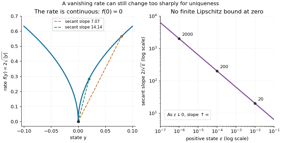
The rate law tends to zero as , but its secant slopes from zero are unbounded:No finite local Lipschitz constant exists at zero. At the quotient is , even though the rates are shrinking to zero. Continuity controls the rate itself; Lipschitz continuity would control its change relative to the state displacement.
There is also a numerical lesson. The forward Euler method starting exactly at zero gives at every step. It reproduces the constant solution of a differential equation for every positive step size, while the moving trajectories remain equally valid. A computation producing one trajectory cannot establish uniqueness. Likewise, the separable differential equation calculation that divides by only describes the moving pieces: checking the original equation recovers the zero pieces and their joins.
For the autonomous differential equation , the real solutions are nondecreasing and lie in . On each nonconstant interval, separation of variables gives , so the solution crosses from to in exactly time . Every nonconstant solution on the entire real time axis is consequentlyfor some real . The two constant solutions complete the list; solutions on shorter intervals are restrictions of these. At the joins both the derivative and the right-hand side are zero, so these are continuously differentiable functions. The right-hand side is continuous but fails Lipschitz continuity at both endpoints, allowing arbitrary waiting time at before departure. Once reaches , monotonicity forces it to stay there. The sine representation without the nonnegative-cosine restriction would incorrectly introduce decreasing pieces.
Articles by others on the same topic

The Peano existence theorem, often referred to in the context of ordinary differential equations (ODEs), is a fundamental result that provides conditions under which solutions to certain initial value problems exist.


