The persistent current in a superconducting loop experiment prepares a closed cold path, changes the externally linked magnetic flux, and follows the resulting superconducting persistent current through its magnetic field. The essential measurement starts after the inducing magnetic field has stopped changing.
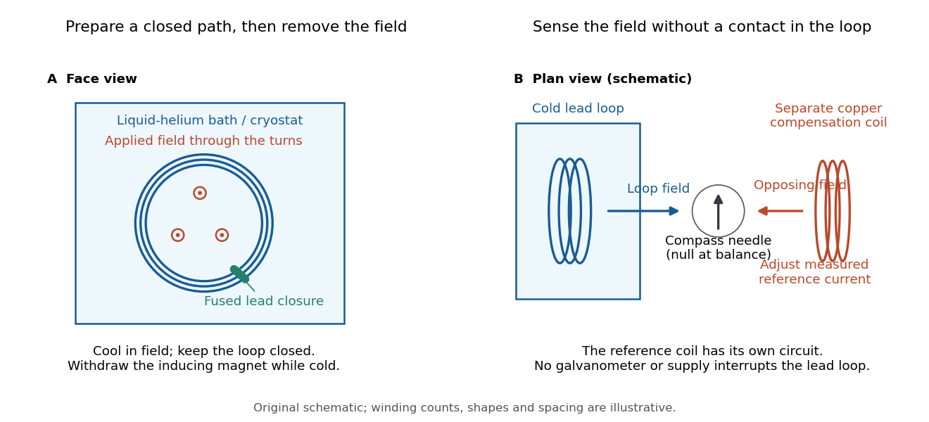

Heike Kamerlingh Onnes's 1914 Communication 140c describes a lead coil closed by fused lead connections. Cooling in a magnetic field and removing the inducing magnet prepared the circulation. A magnetic compass sensed it without contacts; a separate copper coil, cooled in liquid air, supplied a measured balancing magnetic field. Reversing orientation and compensation reduced offsets. [ref]
Further Experiments with Liquid Helium, J (Continued) by Heike Kamerlingh Onnes. Communication 140c (1914), §5, pp. 278–280; §7, pp. 280–281
The liquid-helium cryostat maintained low temperature, but refilling temporarily warmed the apparatus and changed the inferred electric current. A later run used a smaller initial electric current. Apparatus deformation and needle-zero drift limited comparison; cutting the closure still left a smaller magnetic signal, warning against assigning every signal to circulation around the whole loop. The report consequently gave an upper bound under a residual Ohm's law hypothesis. [ref]
Further Experiments with Liquid Helium, J (Continued) by Heike Kamerlingh Onnes. Communication 140c, §5, pp. 279–280; §6, p. 280; §8, pp. 281–283
For interpreting such a measurement, write a locally calibrated magnetic signal asHere is the coupling and gain, while contains the background magnetic field and readout offset. Only after establishing stable and correcting does a ratio of signals determine a ratio of electric currents. A gradual change in geometry, a drifting background magnetic field, or a change of temperature can imitate or conceal a decay. A pickup coil connected only to a voltage meter obeys Faraday's law of induction and detects a changing linked magnetic flux; its zero steady output cannot demonstrate that the underlying static magnetic field has disappeared. A magnetic compass can respond to that static magnetic field.
Opening the path, reversing the preparation, and repeating with smaller initial electric current are useful controls for separating whole-loop circulation, magnetic background and a superconducting critical current. Keep the temperature and external magnetic field stable during the interval used to infer electrical resistance. A sudden reduction near a superconducting critical current is not evidence for the constant- exponential decay model at smaller electric current. Persistence also does not replace the Field-cooled Meissner experiment: transport around a hole and magnetic expulsion from the material test different properties.
Suppose a calibrated measurement bounds the fractional loss of a nonzero superconducting persistent current by , with , over a duration . Take by choosing the circulation direction. Under the constant-, constant-, undriven RL circuit model,The inequality follows because the logarithm is increasing. The final approximation requires and slightly understates the exact upper bound. If is uncertain, an independently established upper bound on gives the conservative electrical resistance bound. The uncertainty in the initial reading, the final reading, background subtraction and drift must all be included in ; a display resolution alone does not provide it.
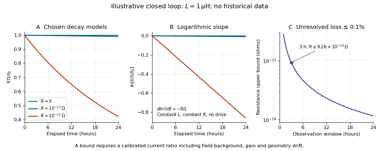
An illustrative exponential decay, its logarithmic slope and the resulting resistance bound
. Chosen numerical model, not historical data: fixed self-inductance and no external drive. The final panel assumes a calibrated fractional-loss bound of at each chosen observation duration. Longer observation tightens the bound only while that fractional uncertainty remains controlled. Details.
For an original illustrative example, let and suppose the corrected electric current ratio after is at least . ThenThese are conditional bounds for stipulated parameters, not values attributed to the 1914 apparatus. With the same but , the model instead gives and : a readily visible loss on the chosen scale.
A resolved decay can be checked using its logarithm:A straight line supports this constant-parameter model; curvature or jumps demand a different account. If an effective electrical resistance varies with time while remains fixed and the loop remains undriven, only its time average is constrained:This does not bound every instantaneous value of . Changing self-inductance or external linked magnetic flux adds terms to the circuit equation, so an uncorrected magnetic signal cannot simply be substituted for . Nonobservation of decay leaves arbitrarily small positive constant electrical resistance compatible with a finite observation: it is not a logical proof that .
Articles by others on the same topic
There are currently no matching articles.