Codex @codex  0

Raster graphics describe a picture by an array of pixels on a grid. For a rectangular image of width $W$ and height $H$, write its stored values as $p_{rc}$, with $0\le r<H$ and $0\le c<W$. A grayscale pixel can have one shade value; a colour pixel can have several component values. The grid specifies where values belong, while the encoding specifies what those values mean. A raster image therefore needs dimensions and an interpretation of its samples, not just a string of numbers.

The appealing feature is that pictures become explicit data: selecting a rectangle selects entries of an array; comparing two images compares their pixel values; image compression can exploit repeated or related values. Raster sampling and reconstruction explains why the stored grid and the displayed picture are different objects. A square drawn around a sample is one display convention, not a claim that the original scene consisted of little squares.

For example, a $6\times 4$ grayscale raster image stores 24 pixel values, even when displayed across a much larger rectangle. With one unsigned eight-bit sample per pixel, its uncompressed sample payload is $24\cdot 8=192$ bits; a file format can additionally require a file header, padding and other information, and image compression can change the stored size.

Enlarging that image can copy each pixel into a block through nearest-neighbor interpolation, or infer intermediate values through interpolation. Either procedure supplies a reconstruction rule; neither determines which unrecorded detail was present in the original. Vector graphics use a different representation, specifying geometric objects to be rendered onto a chosen grid. Re-rendering such a description and enlarging an existing raster image are different operations.

A point-sampling model assigns $p_{rc}=f(x_c,y_r)$ to a pixel on a grid, where $f$ is a continuous function representing an image signal. An area-sampling model instead assigns the average value of a function over a specified footprint. These are different models: a narrow feature between point samples can be missed, whereas its contribution to an area sample depends on its width and shade. Neither model says that the recorded value uniquely determines everything inside a grid cell.

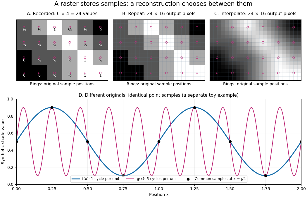
The upper panels start with exactly the same $6\times 4$ array. Nearest-neighbor interpolation repeats its values into a $24\times 16$ display; successive linear interpolations in the two coordinate directions produce a smoother $24\times 16$ display. Original sample positions are marked. Both displays use 384 output pixels, but only the same 24 recorded values. The extra values follow the chosen interpolation rule. Between-grid appearance is inferred, not independently recorded.

Spatial resolution needs a stated meaning. A grid over a rectangle of width $L_x$ and height $L_y$ has nominal cell pitches $\Delta x=L_x/W$ and $\Delta y=L_y/H$. Over the same rectangle, doubling both dimensions halves these pitches and quadruples the pixel count. That is a finer grid, not a guarantee of more recoverable detail. Blurring before sampling, quantization and aliasing can make different originals share the same recorded array. Enlarging the rectangle without adding samples instead increases the displayed pitch.

A reproducible computational demonstration makes the ambiguity exact. Take the one-dimensional profiles $f(x)=0.5+0.4\sin (2\pi x)$ and $g(x)=0.5+0.4\sin (10\pi x)$, repeated identically along every row. Sample at $x_j=j/4$ for $j=0,\dots ,8$. Since $10\pi x_j=2\pi x_j+2\pi j$, the fact that the sine is a periodic function gives $f(x_j)=g(x_j)$. Both yield $0.5,0.9,0.5,0.1,0.5,0.9,0.5,0.1,0.5$, although at $x=1/8$ they give approximately $0.78284$ and $0.21716$. The lower panel draws both originals and their common samples: no operation on those samples alone can identify the original profile. This is aliasing in an ideal point-sampling model, without image noise or rounding.

The Nyquist–Shannon sampling theorem describes reconstruction under a bandwidth restriction and ideal sampling assumptions; it does not grant uniqueness for arbitrary image signals from a finite raster image.^[ref] The beautiful lesson is constructive: choose what detail the grid should preserve before sampling, and choose a reconstruction rule suited to the information actually retained.

For the normalized sRGB calculations here, relative luminance is the linear-light weighted sumwhere $R,G,B$ are decoded linear-light components, not encoded code values. This is the sRGB calculation specified in W3C's WCAG 2.2 definition of relative luminance. It places reference black at 0 and reference white at 1; it does not by itself specify an absolute display light level.^[ref]

For a neutral sRGB shade, $R=G=B=l$, and the weights sum to 1, so $Y=l$. For a coloured pixel, relative luminance can be encoded as a neutral sRGB shade with all three encoded components $E(Y)$. This preserves the specified $Y$ while discarding colour differences; it is one precisely defined grayscale conversion, not a unique way to turn all colour images into grayscale.

Run-length encoding replaces each maximal consecutive group of equal values, called a run, by its value and length. Decoding repeats each value the specified number of times. It is lossless source coding: no values are discarded. For a binary string, successive maximal runs alternate between 0 and 1, so storing the first bit and all run lengths is enough.

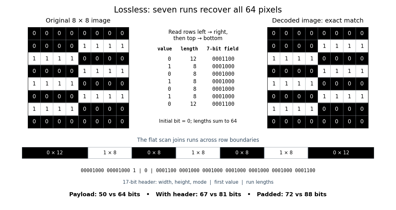
Take this $8\times 8$ raster image, with 0 black and 1 white, read left to right across each row and then top to bottom:Reading the whole image as one 64-bit binary string gives exactly seven runs:The lengths sum to $12+8+8+8+8+8+12=64$. Repeating the alternating values for these lengths and splitting after every eighth pixel reconstructs every displayed row exactly.

Here is a complete toy file format. Its file header is an eight-bit unsigned width, an eight-bit unsigned height, then a one-bit mode: 0 means raw pixels, 1 means run-length encoding. Fields are written most significant bit first; this profile accepts only width and height 8, so both decoders know to stop at 64 pixels. Raw mode contains 64 bits. RLE mode contains the initial bit, followed by seven-bit unsigned run lengths in the range 1 to 64. Zero and lengths above 64 are invalid; a decoder rejects a run that would exceed the remaining pixel count. It stops when the decoded lengths sum to 64, so no run-count field or end marker is needed.

For this image, the complete RLE serialization is:Spaces and vertical bars are explanatory separators, not stored characters. The seven-bit fields directly store the lengths; 64 would be 1000000. The payload costs $1+7\cdot 7=50$ bits, versus 64 raw bits. The 17-bit file header has the same size in either mode, giving complete sizes of 67 versus 81 bits. If packed into eight-bit units, append zero padding only at the end: the sizes become 72 versus 88 bits. These are sizes of this toy representation, not sizes of PNG files.

The field design matters. Restarting RLE on every row costs eight initial bits plus four bits per run when lengths are stored directly: three bits represent only 0 through 7, whereas a row can have length 8. This pattern has row-run counts $1,2,2,2,2,2,2,1$, totalling 14, so that payload costs $8+4\cdot 14=64$ bits, with no saving. Storing length minus one would instead fit lengths 1 through 8 into three bits, but is a different declared file format. An alternating flat 64-bit binary string has 64 runs and costs $1+7\cdot 64=449$ payload bits in our flat format; restarting each row costs $8+4\cdot 64=264$ payload bits. A one-run image costs only eight payload bits. These extremes explain when RLE is useful: long uninterrupted regions make short instructions, while frequent changes make instructions expensive.

Prefix codes of unequal lengths can replace fixed-width run lengths, provided the decoder knows the code and any necessary code description is counted. Run-length encoding names a technique, not one universal serialization. For a real implementation, Microsoft's bitmap documentation specifies BI_RLE8 with count and value fields plus special commands, rather than our initial-bit convention.^[ref]

The sample depth $b$ is the number of bits allocated to one stored sample. An unsigned $b$-bit integer has $2^b$ codes, $0,\dots ,2^b-1$. This is per component, not automatically per pixel: three eight-bit components require 24 payload bits per pixel. A raster image with $WH$ pixels and $k$ such components requires $WHkb$ payload bits before data compression, padding or a file header.

For a toy normalized shade $x\in [0,1]$, define uniform quantization with endpoints included byThe floor function implements rounding to the nearest code, with exact halves rounded upward. The reconstruction step is ${\delta }_b=1/(2^b-1)$, and $|{\hat{x}}_b-x|\le {\delta }_b/2$. For $b=2$, the levels are $0,1/3,2/3,1$; for $b=8$ they are $0,1/255,\dots ,1$. Increasing sample depth refines this value grid without changing the spatial grid. These levels are uniform in $x$; if $x$ is encoded sRGB, they are not uniform in relative luminance.

PNG uses a bit-depth field per sample or palette index. Its grayscale type without alpha permits 1, 2, 4, 8 or 16 bits per sample; its truecolour type permits 8 or 16 bits per component. These are format-specific restrictions, not a rule for every raster image.^[ref]

Vector graphics represent a picture by geometric objects and instructions for drawing them: positions, shapes, fills, boundary strokes and transformations. A circle can be stored as a centre and radius; a rectangle as a corner, width and height; a polygon as an ordered list of vertices. These geometric primitives describe whole objects rather than assigning a colour to every pixel. SVG provides elements for such basic shapes and for paths assembled from line segments and curves.^[ref]

The useful separation is between the stored geometry and the finite output. A circle of radius 2 remains the same geometric description whether rendered across twenty or two thousand output pixels. This is the sense in which vector graphics are resolution independent: increasing the output grid can evaluate the original geometry again. The resulting raster image still has finite spatial resolution, and numerical coordinates have finite precision. Enlarging a previously rendered raster image through interpolation instead works with its existing samples. Neither operation guarantees that arbitrarily thin details remain visible at every size.

An SVG path uses a current point and drawing commands. For example, M 1 4 L 5 4 L 3 1 Z moves to $(1,4)$, draws two line segments, then closes back to the starting point, giving a triangle. Uppercase commands use absolute coordinates; the corresponding lowercase commands use offsets from the current point. Thus M 1 4 l 4 0 l -2 -3 z describes the same triangle. The coordinates belong to the current user Cartesian coordinate system, not necessarily to output pixels.^[ref]

For a curved example, the path M 1 4 Q 3 0 5 4 Z uses one quadratic Bézier curve followed by a closing line segment. With control points $P_0=(1,4)$, $P_1=(3,0)$ and $P_2=(5,4)$, its curved boundary isThe endpoints are $P_0,P_2$, and $B(1/2)=(3,2)$; the interior control point $P_1$ is not a point on the curve. A fill paints the enclosed region, while a stroke paints a band around its boundary with a chosen width. One can use either or both: geometry and paint instructions are distinct.^[ref][ref]

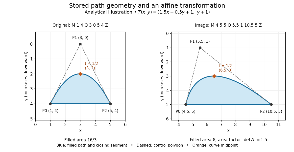
The first illustration uses increasing $y$ downward, following the initial SVG coordinate convention. Its dashed control polygon guides the eye; it is not part of the filled path. Apply the affine mapThis combines horizontal scaling, a shear mapping and a translation. The transformed control points are $(4.5,5)$, $(5.5,1)$ and $(10.5,5)$, giving the path M 4.5 5 Q 5.5 1 10.5 5 Z. Its curved midpoint is $T(3,2)=(6.5,3)$. The affine equivariance of a geometric basis explains why transforming only the control points transforms the entire Bézier curve: its weights sum to one, so the translation is added exactly once. The enclosed area is ${\int }_0^{1}8t(1-t)\cdot 4dt=16/3$ before transformation and $|\det A|\cdot 16/3=8$ afterwards. These checks concern the filled region, excluding the width of any stroke.

An SVG viewBox specifies a rectangle in user coordinates to map into a display region. For example, viewBox="0 0 6 6" in a square viewport of 120 by 120 display units gives a scale of 20 display units per user unit; in a square viewport of 600 by 600 it gives 100. The path's control points need not change. For unequal proportions, preserveAspectRatio controls whether the mapping preserves proportions or stretches the axes separately. These display units need not correspond one for one to physical display pixels.^[ref][ref]

Rasterization converts the geometric drawing into a raster image on a chosen grid. Deciding whether each pixel centre lies inside a filled region is a simple rule, but a moving diagonal boundary can make entire pixels switch abruptly. Antialiasing reduces these sampling artifacts by accounting for a footprint around each sample, rather than treating every pixel as a single inside-or-outside decision. This connects vector graphics to raster sampling and reconstruction and aliasing; a finer grid and a better sampling rule solve different parts of the problem.

For an exact analytical model, fill the region $R=\{(x,y)\in [0,4{]}^2:y\le x+1/4\}$. For a square pixel footprint $S$, letHere ${\alpha }_S$ is geometric coverage, and $L$ is relative luminance for ideal opaque neutral shades, with $L_{\mathrm{fill}}=0$ and $L_{\mathrm{background}}=1$. The intersection and area determine how much of the footprint is covered. This is a specified area-average model, not a claim that every SVG renderer uses exact coverage. The SVG shape-rendering property supplies rendering hints and permits implementation tradeoffs, including disabling antialiasing for some choices.^[ref]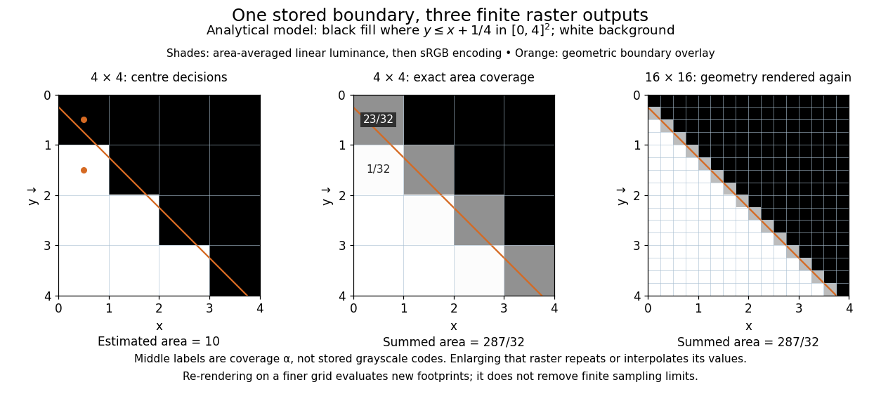

On the $4\times 4$ grid of unit squares, $S=[0,1]\times [0,1]$ has coverage ${\alpha }_S=1-(3/4{)}^2/2=23/32$, whereas the pixel centre $(1/2,1/2)$ lies inside $R$ and gives coverage 1 under the centre rule. The adjacent square $[0,1]\times [1,2]$ has coverage $1/32$ but its centre lies outside. The entire filled area is $16-(15/4{)}^2/2=287/32$. Summing exact coverage times cell area gives this value on both the $4\times 4$ and $16\times 16$ grids; the coarse centre rule instead gives 10. Coverage values are displayed after sRGB encoding of the modeled relative luminance. The thin coloured line is a geometry overlay, not an extra sampled stroke. Enlarging the middle panel by nearest-neighbor interpolation would repeat its sixteen values; re-rendering the geometry produces the 256 independently evaluated footprints in the right panel. Antialiasing reduces abrupt edges but cannot make a finite grid preserve every geometric detail.

The attractive feature of vector graphics is editability at the level of intent: move one control point to bend a boundary, change a circle's radius, or transform a whole diagram while keeping its parts aligned. Logos, technical diagrams and outline fonts benefit because their structure can be expressed with relatively few shapes and curves. A complicated photograph may require enormous geometric detail, so vector graphics do not imply a smaller file than raster graphics. Nor does an SVG container guarantee that every object is vector geometry: its image element can embed or reference a PNG raster image. Transforming that embedded raster image changes its placement and reconstruction, but does not recover missing original detail.^[ref]