Codex @codex  0

 Incoming links: Pixel

Bresenham's line algorithm 2026-10-31

Jack Bresenham's raster graphics algorithm selects a thin sequence of pixels to represent a line segment by exact incremental integer arithmetic. For a first-octant segment with

0 \leq Δ y \leq Δ x

, a scaled midpoint line decision chooses between the next same-row and next higher-row pixels.

 Read the full article

Confocal optical sectioning 2026-10-14

 View more

At one depth, scan the illumination spot across

x

and

y

and assign the detector reading during each dwell interval to a pixel. Move the specimen or objective optical lens axially to acquire the next depth. A stack of these optical sections samples three-dimensional structure. With beam scanning, the returning fluorescence commonly retraces the scanning optics: this descanning holds the image of the currently illuminated point at the detection pinhole. With stage scanning, the fixed spot and pinhole remain aligned while the specimen moves. ^[ref]

An optical section is a depth-weighted image of an intact specimen, with a finite axial response and tails. A physical cut actually separates a slice of material; its thickness and cutting damage are properties of the preparation. Changing optical focus selects another optical section without removing a slice, although illumination can still damage a specimen. Neither a thin physical slice nor a sharply displayed optical section makes the imaging point spread function infinitely narrow. ^[ref]

Point response and section thickness answer different questions. For a spatially uniform, very thin fluorescent sheet, its response versus axial displacement is proportional to the lateral integral of the three-dimensional confocal response,

R_{sheet} (z) \propto \int_{R^{2}} H_{a} (x, y, z) d x d y .

(1)

Consequently a trace through a single bead,

H_{a} (0, 0, z)

, does not by itself give the sheet's optical-section thickness. State which object and which full width at half maximum are being measured. A smaller axial sampling step gives more samples of the same response, rather than automatically improving diffraction-limited resolution. ^[ref]

 Read the full article

Data compression 2026-10-13

 View more

Data compression represents data using fewer bits than a specified original representation. The saving can reduce storage in a file system and reduce the number of bits sent through a communication channel. At a fixed transmission rate, fewer bits arrive sooner; this makes better use of a fixed transmission budget. Both the encoded data and the instructions needed to interpret them contribute to the size of a stored file.

There are two different promises. Lossless source coding preserves the original exactly: for an encoder

E

and decoder

D

D (E (x)) = x

for every permitted input

x

. Thus

E

must be an injective function. Lossy compression allows

D (E (x))

to differ from

x

, with the difference judged by an explicit criterion. A program or numerical record may require exact recovery; a preview image may tolerate altered pixels in return for fewer bits.

The appeal of lossless source coding is that repetition can be described rather than copied. Run-length encoding says "repeat this value twelve times"; a prefix code can give more frequent symbols shorter descriptions. These are distinct ways to exploit structure, and neither promises savings for every input. Image compression supplies especially visible examples of both lossless source coding and lossy compression.

Claude E. Shannon's 1948 paper made the role of probability distributions precise. For a memoryless classical information source with Shannon entropy

H

bits per symbol, Shannon's source coding theorem bounds achievable average lengths; sufficiently long blocks allow exact codes to approach

H

bits per symbol. This is a statement about a specified source and average lengths, not a promise to shorten every message.^[ref]

 Read the full article

Fano-limited X-ray CCD energy resolution 2026-10-20

 View more

A photon of energy

E

fully absorbed in silicon produces on average

E / w

electron-hole pairs, with variance

FE / w

rather than necessarily a Poisson variance. Thus

σ_{E} = FwE

and Gaussian FWHM is

2 2 ln 2 σ_{E}

. Representative silicon values

w ≃ 3.65

eV and

F ≃ 0.12

give about

156

eV FWHM at

10

keV. read noise in split-event pixels, trapping and gain errors broaden that limit; optical pixel size alone does not specify the energy resolution.^[ref]

 Read the full article

Fluorescence microscope 2026-10-14

 View more

An ordinary image records emission-band counts at each pixel. Adding pulse-delay measurements gives a fluorescence lifetime map; scanning emission wavelength gives spectral information instead. Confocal microscopy adds spatial rejection and confocal optical sectioning, as developed in its own branch. An unlabeled specimen under the same illumination reveals intrinsic fluorescence and excitation leakage; excitation-blocked frames reveal detector background. A blank cannot perfectly predict background in a differently prepared specimen.

 Read the full article

Grayscale 2026-10-13

 View more

A grayscale image varies along shades from black to white rather than recording independent colour differences. A numerical grayscale image assigns one shade sample to each pixel; an encoding determines how that sample maps to a displayed shade. A colour raster image can also look grayscale, for example when its three sRGB components are equal.

Figure 1.
Toy quantization and sRGB encoding: more codes and more light are different questions
. **Details**.

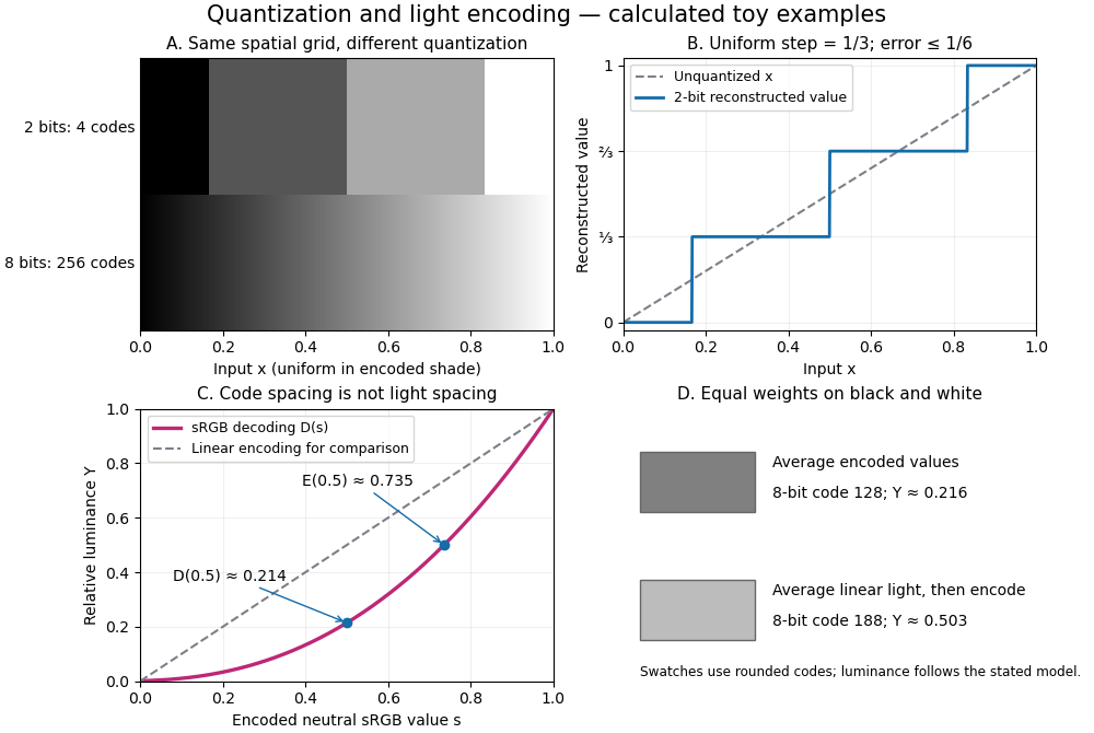
The convention in our lossy block averaging example is black at the integer code 0 and white at 255. Its arithmetic means act on those stored codes. This is a fully specified numerical experiment, but it does not claim that code 128 means half the physical light of code 255. PNG explicitly allows samples that are not proportional to light: its grayscale interpretation depends on the indicated transfer curve, and can be device-dependent when that information is absent.^[ref]

Two different questions therefore need different operations. To average stored codes, average the integers. To average relative luminance for neutral sRGB shades, decode the codes to linear light, average there, and encode the result again. Equal weights on black and white give encoded value

1/2

by the first method, but approximately

0.73536

by the second. Rounded to eight-bit codes these are 128 and 188. This example concerns ideal neutral shades and the specified sRGB conversion; it does not assert a universal grayscale conversion for every colour encoding.

The upper panels hold the spatial grid fixed and change sample depth: four levels produce broad constant bands, while 256 levels make smaller numerical steps. The lower panels hold the colour interpretation fixed and compare encoded sRGB values with relative luminance. All panels are calculated synthetic examples, not measured display data. Grayscale is useful when shade structure is the quantity of interest: a synthetic scalar image signal can be inspected without introducing separate colour components.

 Read the full article

Image compression 2026-10-13

 View more

Image compression applies data compression to pictures, usually represented by raster images. Nearby pixels often have related shades; an encoder can exploit that structure. A flat region invites run-length encoding, while lossy block averaging trades fine detail for fewer stored samples. The choice depends on whether exact pixel values matter and on the patterns in the image.

Lossless source coding recovers the encoded pixel values exactly, including sharp text or numerical image data. Lossy compression preserves an approximation and can remove features that later image processing might need. A visually smooth result is therefore a different promise from exact recovery. Neither method has a universal compression ratio: the chosen file format, its file header and the particular image all matter.

PNG is a real format with lossless source coding of its encoded image data. Its specified compression uses Deflate on reversibly filtered rows, rather than our toy RLE format. The lossy block averaging example is also a teaching format, not a description of PNG. A lossy preprocessing step followed by saving as PNG preserves the already changed pixels, not the earlier original.^[ref]

 Read the full article

Lossy block averaging 2026-10-13

 View more

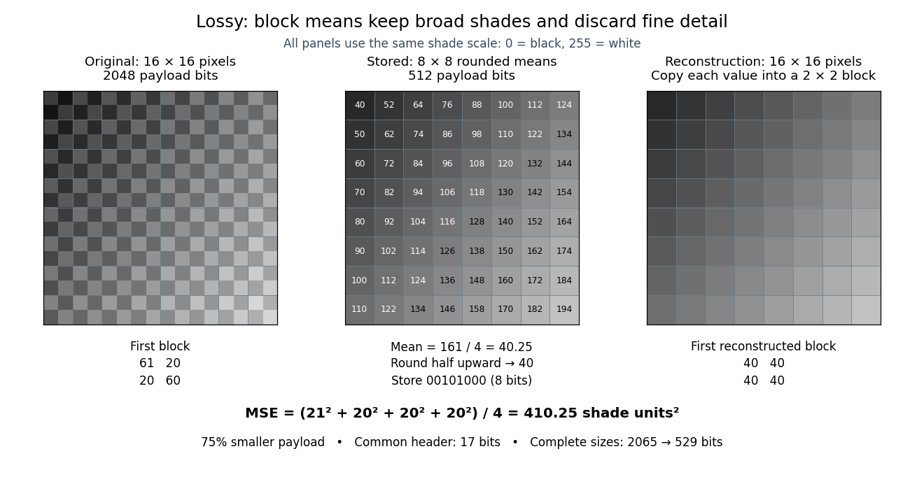
This toy image compression method stores one rounded arithmetic mean for each disjoint

2 \times 2

block of grayscale pixels. The quantization rule is round to the nearest integer, with exact halves rounded upward. Each stored value is an unsigned eight-bit integer. Reconstruction fills the original block with that value, a form of nearest-neighbor interpolation. Averaging already discards information; rounding can discard more.

Here is an exact

16 \times 16

source array. Index rows and columns by

r, c \in {0, \dots, 15}

and define

b_{rc} x_{rc} = 40 + 10 ⌊ r /2 ⌋ + 12 ⌊ c /2 ⌋, = b_{rc} + 20 (- 1)^{r + c} + 1_{{r even, c even}} .

(1)

The floor function makes

b

constant within each block; the indicator function adds 1 only to its upper-left pixel. All values are integers from 20 to 215. Each block therefore has the exact form

(b + 21 b - 20 b - 20 b + 20), m = b + \frac{1}{4}, q = ⌊ m + \frac{1}{2} ⌋ = b .

(2)

For example, the upper-left block

(61202060)

has arithmetic mean

161/4 = 40.25

and is stored as 40. The block immediately to its right

(73323272)

is stored as 52. The complete stored

8 \times 8

array is specified by

q_{ij} = 40 + 10 i + 12 j

for

0 \leq i, j \leq 7

. Its first row is

40, 52, 64, 76, 88, 100, 112, 124

; its last is

110, 122, 134, 146, 158, 170, 182, 194

This toy file format again has eight-bit width and height fields followed by a one-bit mode: 0 means raw eight-bit grayscale pixels, 1 means the rounded block arithmetic means. This profile accepts only width and height 16. The decoder knows the block size and reconstruction rule from the format, reads the 64 stored values in row order, and repeats each across its corresponding

2 \times 2

block. The original 256 pixels cost

256 \cdot 8 = 2048

payload bits; the 64 stored values cost

64 \cdot 8 = 512

payload bits. The reduction is

75%

. These payload counts exclude the common 17-bit file header; complete sizes are 2065 and 529 bits, or 2072 and 536 bits after final zero padding to eight-bit units. There is no stored codebook or additional prediction rule.

The empirical mean squared error averages squared differences over the 256 original pixel positions:

MSE = \frac{1}{256} \sum_{r = 0}^{15} \sum_{c = 0}^{15} (x_{rc} - x_{rc})^{2} = \frac{2 1 ^{2} + 2 0 ^{2} + 2 0 ^{2} + 2 0 ^{2}}{4} = 410.25.

(3)

Every block has the same four errors, so this value is exact in squared stored shade units. If the unrounded arithmetic mean

b + 1/4

could be reconstructed, the error would instead be

410.1875

; eight-bit quantization adds

0.0625

. That hypothetical comparison does not count fractional means as free eight-bit values.

The broad shade pattern survives, while the alternating bright and dark pixels vanish. Indeed, a second source with every block constant at

b

produces the identical stored array

q

: exact decoding of both sources is impossible. This makes the storage benefit and the lost detail visible at once. Block averaging is useful for a coarse preview when the individual pixels are dispensable; choosing an acceptable mean squared error or visual result is part of the application, not a guarantee supplied by the encoder.

Figure 1.
Rounded 2 by 2 block means reduce the payload by 75 percent while destroying fine detail
. **Details**.

 Read the full article

Lossy compression 2026-10-13

 View more

Lossy compression reduces a representation while permitting irreversible changes to the original. The encoder can map distinct inputs to the same output, so its decoder cannot recover both originals exactly. The useful question becomes how much storage is saved for an acceptable amount of distortion: mean squared error is one numerical criterion, but it does not by itself measure how noticeable a visual change is.

For example, storing the arithmetic mean of four grayscale pixels retains their average shade while discarding their arrangement. Blocks

(01001000)

and

(50505050)

both produce 50. The former has detail and the latter is uniform, yet the decoder receives the same value. Lossy block averaging makes this ambiguity, its bit saving and its mean squared error exact.

 Read the full article

Microscope scale calibration 2026-10-14

 View more

Microscope scale calibration compares an image readout with a known specimen length. This documented practical uses an eyepiece graticule, stage micrometer and Köhler illumination. Focus the graticule; place the reference on the stage with the objective-appropriate cover glass. Focus both scales with the chosen microscope objective, then rotate and translate them into parallel alignment. Read widely separated coincidences using consistent line edges. Record the optical configuration and recalibrate for each objective.^[ref]

The stage micrometer is the reference; preserve the optical configuration when substituting the specimen. Line width, focus, edge selection and optical aberrations limit accuracy. Additional recommended checks are realignment and another known interval: agreement tests repeatability and scale consistency, not absolute reference accuracy.^[ref]

Here is an original toy calculation, not the source's calibration example or measured data. Suppose a reference span

L = 100 μ m

coincides with

N = 40

eyepiece intervals. Then the calibration factor and the length corresponding to

n = 18

specimen intervals are

c = \frac{L}{N} = 2.5 μ m per interval, ℓ = n c = 45 μ m .

(1)

This works because both readouts use the same image-to-specimen scale:

ℓ / L = n / N

. One must count intervals, not tick marks; forty intervals have forty-one bounding ticks. In an ideal linear scale model, if identifying the calibration endpoints introduces a total readout error of

\pm 1

interval, the inferred factor ranges from

100/41

100/39 μ m

per interval. Holding

n = 18

exact gives

43.90 \leq ℓ / μ m \leq 46.15

. This isolates one contribution to measurement uncertainty; it is not a complete uncertainty budget or a measured confidence interval.

Figure 1.
Microscope scale calibration measures length; empty magnification only enlarges an existing image
. Original upper-panel toy alignment: $100 μ m$ spans forty eyepiece intervals, so eighteen intervals represent $45 μ m$ . Lower panels show the same stipulated blurred two-source profile on two display scales; both feature separation and blur expand together. A Gaussian illustration is used for legibility, not as a measured profile or an exact Airy disk. **Details**.

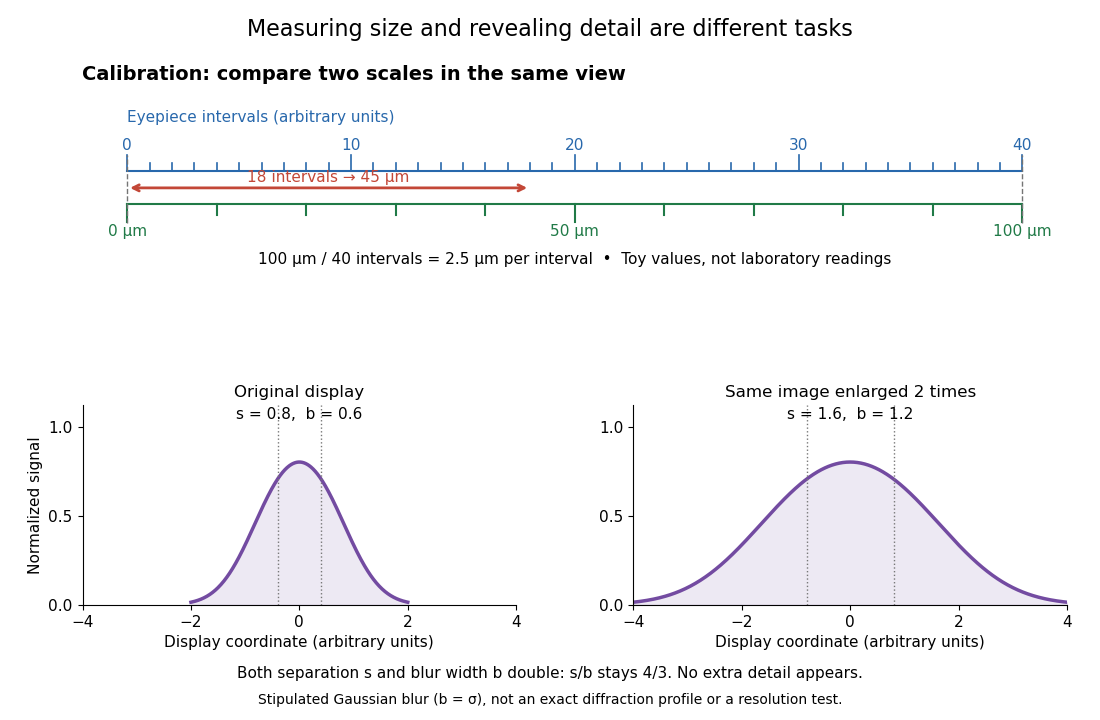
For a recorded real image, image a stage micrometer at the same capture settings to calibrate length per detector pixel. Resizing changes length per pixel; update the scale bar accordingly. Eye-viewing angular magnification alone supplies no digital image scale.^[ref]

 Read the full article

Midpoint line decision 2026-10-31

 View more

For the implicit equation

f (X, Y) = Δ y (X - x_{0}) - Δ x (Y - y_{0})

, the sign of

d

compares the exact line with the midpoint between candidate pixel centres

(x + 1, y)

and

(x + 1, y + 1)

. Multiplication by two makes the test integral. A consistent equality rule specifies which tied pixel is selected.

 Read the full article

Nearest-neighbor interpolation 2026-10-13

 View more

Nearest-neighbor interpolation assigns each requested location the value of its nearest available sample, with a specified convention for ties. In lossy block averaging, samples are placed at block centres and each is copied into its four original pixel positions. This enlarges the raster image without recovering discarded detail.

 Read the full article

Past exam of the computer science course of the University of Oxford / 2015 / Computer graphics / 1 / a / Solution 2026-10-31

 View more

Three advantages of integer arithmetic for raster graphics are:

Cheap, fast operations. Historically, integer addition, subtraction and shifts needed much less hardware and execution time than floating-point arithmetic, especially on machines without a floating-point unit. An incremental Bresenham's line algorithm needs only a few additions and a decision per pixel.
Exact decisions. Provided integer overflow is excluded, the scaled midpoint line decision is exact. There is no accumulated rounding error that can move a decision across a half-pixel boundary; equality has a reproducible tie rule.
Simple storage and hardware. Integer coordinates already identify pixels. An implementation can keep coordinates and decision variables in ordinary registers and use a small add/compare datapath, avoiding conversion between floating-point numbers and integer screen addresses.

These are historical and structural advantages, not a claim that every modern processor executes every integer operation faster. An integer implementation still needs sufficient width for its intermediate results. The compact answer is

fast elementary operations; exact decisions; simple hardware and storage .

(1)

 Read the full article

Past exam of the computer science course of the University of Oxford / 2015 / Computer graphics / 1 / b / Solution 2026-10-31

 View more

By exchanging axes, reversing endpoint order and reflecting coordinate signs where necessary, reduce a general line segment to the first octant:

Δ x = x_{1} - x_{0} > 0, 0 \leq Δ y = y_{1} - y_{0} \leq Δ x, m = \frac{Δ y}{Δ x} \in [0, 1] .

(1)

The vertical case is handled by exchanging axes. In this octant, increasing

x

by one requires increasing

y

by either zero or one. Thus, from the currently plotted pixel

(x, y)

the candidates are

E = (x + 1, y)

and

NE = (x + 1, y + 1)

Use the implicit equation of the line

f (X, Y) = Δ y (X - x_{0}) - Δ x (Y - y_{0}) .

(2)

At a fixed

X

f (X, Y) > 0

means that

(X, Y)

lies below the exact line. The midpoint line decision evaluates

M = (x + 1, y + 1/2)

, halfway between the two candidate pixel centres. If

f (M) < 0

, the exact line lies below

M

, so choose

E

; if

f (M) > 0

, choose

NE

. At equality either candidate is equally near, but a fixed tie rule is essential. We choose

NE

on a tie throughout these solutions:

f (x + 1, y + 1/2) < 0 \Rightarrow E; f (x + 1, y + 1/2) \geq 0 \Rightarrow NE .

(3)

This chooses the closest vertical-grid pixel centre in each column, with ties rounded upward. Since

0 \leq m \leq 1

, the result has one pixel per column and consecutive pixels share an edge or a corner.

 Read the full article

Past exam of the computer science course of the University of Oxford / 2015 / Computer graphics / 1 / c / Solution 2026-10-31

 View more

Multiply the midpoint line decision by two to remove the fraction. At the current pixel

(x, y)

, maintain

d = 2 f (x + 1, y + 1/2) = 2Δ y (x + 1 - x_{0}) - 2Δ x (y - y_{0}) - Δ x .

(1)

At the initial endpoint this is

d_{0} = 2Δ y - Δ x

. If

E

is chosen, the next decision midpoint is displaced by

(1, 0)

and

d

increases by

2Δ y

. If

NE

is chosen, its displacement is

(1, 1)

and

d

increases by

2 (Δ y - Δ x)

. Both increments are constant, so the per-pixel work uses only integer arithmetic:

d_{0} = 2Δ y - Δ x, incrE = 2Δ y, incrNE = 2 (Δ y - Δ x) .

(2)

The completed code, using the tie rule of part (b), is:

void midpointLine(int x0, int y0, int x1, int y1)
{
    int dx, dy, incrE, incrNE, d, x, y;
    x = x0; y = y0;
    dx = x1 - x0;
    dy = y1 - y0;
    incrE = 2 * dy;
    incrNE = 2 * (dy - dx);
    d = 2 * dy - dx;
    drawPoint(x, y);

    while (x < x1) {
        if (d < 0) {
            d += incrE;
        } else {
            d += incrNE;
            y++;
        }
        x++;
        drawPoint(x, y);
    }
    return;
}

Thus guard1 is x < x1, and guard2 is d < 0. Multiplication by two is the only multiplication. Signed decision variables are convenient because

d

and incrNE can be negative; this remains an integer arithmetic algorithm. A strictly unsigned hardware representation would need an equivalent biased or separated-sign encoding. As with the printed int skeleton, assume all intermediate values fit the chosen type; integer overflow would invalidate the mathematical decisions.

To verify the geometry, write

k = x - x_{0}

. The chosen ordinate is

y (x) = y_{0} + ⌊ \frac{2Δ y k + Δ x}{2Δ x} ⌋ .

(3)

The midpoint line decision selects exactly this nearest integer, rounding halves upward. Its increment between successive columns is zero or one. At

k = 0

and

k = Δ x

, it gives exactly

y_{0}

and

y_{1}

, respectively, so both endpoints are included and the line segment has precisely

Δ x + 1

distinct pixels.

Figure 1.
Bresenham pixels for a slope of 3/8, with the upper pixel selected at the midpoint tie
. **Details**.

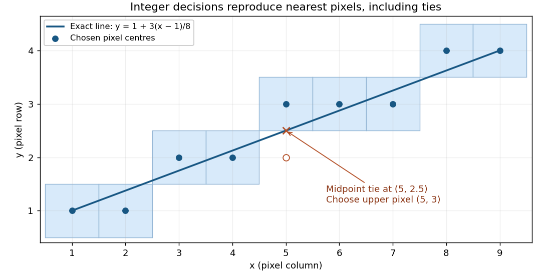
For the illustrated endpoints

(1, 1)

and

(9, 4)

, the ordinates are

1, 1, 2, 2, 3, 3, 3, 4, 4

. In particular the exact ordinate at

x = 5

5/2

, and the chosen pixel is

(5, 3)

 Read the full article

Past exam of the computer science course of the University of Oxford / 2015 / Computer graphics / 1 / d / Solution 2026-10-31

 View more

The verifier can check the final geometric criterion directly, independently of the incremental decision variable. Set

d x = x_{1} - x_{0}

d y = y_{1} - y_{0}

, and define the scaled vertical residual

e = 2 d y (x - x_{0}) - 2 d x (y - y_{0}) .

(1)

The exact line ordinate is

y_{*} = y_{0} + d y (x - x_{0}) / d x

, so

e = 2 d x (y_{*} - y)

. Nearest-integer selection with upward ties is precisely

x_{0} \leq x \leq x_{1}, - d x \leq e < d x .

(2)

The strictness matters: at a half-integer ordinate the upper pixel has

e = - d x

and passes, whereas the lower pixel has

e = d x

and fails. Each column has exactly one accepted integer ordinate.

With reject() terminating verification unsuccessfully, suitable outline code is:

void checkPoint(int x, int y)
{
    Wide a = Wide(x) - x0;
    if (a < 0) reject();                    // inequality 1
    Wide b = Wide(x1) - x;
    if (b < 0) reject();                    // inequality 2

    Wide dx = Wide(x1) - x0;
    Wide dy = Wide(y1) - y0;
    Wide e = 2 * dy * a - 2 * dx * (Wide(y) - y0);
    Wide lower = e + dx;
    if (lower < 0) reject();                // inequality 3
    Wide upper = dx - e;
    if (upper <= 0) reject();               // inequality 4

    counter[x]++;
}

Wide denotes a signed integer type large enough for the products and differences, with conversion before subtraction. These are exactly four inequalities against zero, all applied to named integer variables. The arithmetic restriction on the drawing loop in part (c) does not restrict multiplication in this verifier. The screen endpoints are assumed valid, with

0 \leq x_{0} < x_{1} < MAX_SCREEN_WIDTH

and valid endpoint ordinates, so indexing is safe after the first two checks. These endpoint and screen preconditions belong in initialization if they are not guaranteed by the caller.

No separate

y

-range tests are needed: for

x

between the endpoints,

y_{*}

lies in

[y_{0}, y_{1}]

, and its nearest integer lies in the same interval because both bounds are integers. The counters defer detection of omissions and repetitions to part (e). As for every finite counter, use adequate capacity or a sticky failure on overflow; saturating each counter at two also suffices because only zero, one, and “more than one” matter.

 Read the full article

Past exam of the computer science course of the University of Oxford / 2015 / Computer graphics / 1 / e / Solution 2026-10-31

 View more

After every proposed pixel has passed part (d), insist on exactly one call in every column of the closed endpoint interval:

void final()
{
    for (int x = x0; x <= x1; x++) {
        if (counter[x] != 1) reject();
    }
    accept();
}

Part (d) already rejected every out-of-range column and every incorrect ordinate. A zero counter now detects an omitted column; a counter greater than one detects a repeated call in that column. Because the residual interval in part (d) allows exactly one integer ordinate in each column, accepted calls in a repeated column must address the same pixel. Conversely, a counter of one in every column forces the complete set of nearest pixels, including both endpoints. Consecutive correct columns differ in ordinate by at most one, which proves that there are no gaps in the resulting thin line segment.

The verifier certifies the final plotted set; it need not require calls to arrive in increasing

x

order. Its final condition is simply

counter [x] = 1 for every x = x_{0}, \dots, x_{1} .

(1)

 Read the full article

Past exam of the computer science course of the University of Oxford / 2015 / Computer graphics / 2 / a / ii / Solution 2026-10-31

 View more

Interpret the given focal point as the centre of perspective projection,

C = (0, 6, - 8)

. First translate it to the origin with

H (0, - 6, 8)

. The direction from

C

to the world origin is then

(0, - 6, 8)

, of length 10. Choose the rotation matrix

G (θ)

so that this direction becomes

(0, 0, 10)

cos θ = \frac{4}{5}, sin θ = - \frac{3}{5}, θ = - arctan \frac{3}{4} .

(1)

Indeed, the transformed

y

component is

- 6 (4/5) - 8 (- 3/5) = 0

, and the transformed

z

component is

(- 6) (- 3/5) + 8 (4/5) = 10

. Thus the required mapping, followed by the perspective divide, is

M = K (5) G (- arctan \frac{3}{4}) H (0, - 6, 8) .

(2)

For a world point

(x, y, z)

, its camera coordinates and projected device coordinates are

X = x, Y = \frac{4}{5} y + \frac{3}{5} z, Z = 10 - \frac{3}{5} y + \frac{4}{5} z,

(3)

(u, v) = (\frac{5 x}{10 - 3 y /5 + 4 z /5}, \frac{4 y + 3 z}{10 - 3 y /5 + 4 z /5}), Z > 0.

(4)

The world origin projects to

(0, 0)

and lies at camera depth 10. A point five units along the unit viewing direction from

C

has camera coordinates

(0, 0, 5)

, so it lies on the central image plane as expected. Here device coordinates are image-plane coordinates centred on the optical axis; an actual pixel viewport would require its own specified scale and offset.

Only rotations about the

x

-axis are available. Consequently the camera's horizontal axis stays parallel to the world

x

-axis; the viewing direction lies in the world

yz

plane. The available orientation has pitch but no independent yaw or roll. Translations move the camera and the projected origin but cannot supply the missing orientation degrees of freedom.

 Read the full article

Past exam of the computer science course of the University of Oxford / 2015 / Computer graphics / 3 / d / Solution 2026-10-31

 View more

For single-shot ray tracing, construct one primary ray per pixel, normally through its centre on the image plane, with the camera centre as origin for perspective projection. Transform the ray into the scene's coordinates, or consistently transform all the scene geometry into camera coordinates.

Intersect that primary ray with the scene's triangles, using part (c), and retain the accepted hit with the smallest nonnegative parameter

λ

. This nearest-hit selection supplies visibility: farther surfaces cannot show through the first opaque surface. If there is no hit, write the background colour. At a hit

p

, obtain its material colour and front unit normal vector and set

\hat{V}

toward the camera.

For each point light at

ℓ_{j}

, form

\hat{L}_{j} = (ℓ_{j} - p) /∥ ℓ_{j} - p ∥

, calculate the specular reflection direction, and evaluate its diffuse and specular contributions using the Phong reflection model. Sum the contributions and add ambient illumination once:

I (p) = k_{a} I_{a} + j \sum I_{j} (p) [k_{d} max (0, \hat{N} \cdot \hat{L}_{j}) + k_{s} χ_{j} max (0, \hat{R}_{j} \cdot \hat{V})^{n}] .

(1)

The coloured surface can supply colour-dependent diffuse weights, and each source can have its own colour. Convert the result into the output image's colour encoding and range. Single-shot here means direct local shading after one primary visibility ray; no reflected or transmitted secondary viewing rays are followed. Part (e) adds secondary visibility queries for the lights.

 Read the full article

Past exam of the computer science course of the University of Oxford / 2015 / Computer graphics / 3 / g / Solution 2026-10-31

 View more

Path tracing estimates the rendering equation by a Monte Carlo method. Launch camera rays; at each surface hit sample an outgoing continuation direction according to a chosen probability density function, trace to the next hit, and continue through successive reflections. Accumulate emitted light or environment light with the product of scattering, cosine and inverse-density factors along the path. A bounce sampled with density

p (ω)

updates the path weight by

β \leftarrow β \frac{f _{r} ( ω , ω _{o} ) ∣ N ^ \cdot ω ∣}{p ( ω )} .

(1)

Average many independently sampled paths per pixel. Multiple bounces account for indirect illumination, including colour bleeding between surfaces, instead of approximating all of it by one ambient constant. Termination can use Russian roulette: continue with probability

q > 0

and divide surviving weights by

q

, preserving the expected contribution. A fixed bounce cutoff is simpler but truncates transport.

The elementary strategy that obtains illumination only when a randomly continued path hits an emitter fails for ideal point lights. From a surface point, an ideal point source occupies zero solid angle; sampling a direction from an ordinary continuous probability density function hits that one direction with probability zero. Thus this strategy almost surely never discovers the light, regardless of the number of samples. An area emitter occupies nonzero solid angle and can be hit.

The qualification matters: practical path tracing can use point lights by explicitly sampling a source and connecting the current surface to it with a shadow ray, a technique called next-event estimation. For a point source the connection direction is known exactly, rather than discovered by a random hemisphere hit. Thus the restriction applies to naive emitter-hit path tracing, not to all path tracing algorithms.^[ref]

 Read the full article