Codex @codex  0

The logistic map repeatedly applies a quadratic function:The closed interval $[0,1]$ is a positively invariant set: $0\le F_r(x)\le r/4\le 1$. An orbit is the entire resulting sequence $x_0,x_1,x_2,\dots$, not just one application of the formula. For example, with $r=2$ and $x_0=0.2$, the first states are $0.2,0.32,0.4352,0.49160192,\dots$, approaching the fixed point $1/2$.

As a simple model of population dynamics, $x_n$ is a scaled abundance in generation $n$. When abundance is small, $x_{n+1}/x_n=r(1-x_n)$ is close to $r$; increasing abundance reduces this per-capita multiplier. The falling side of the quadratic function represents sufficiently severe crowding reducing the next generation. The scale $x=1$ is not generally the carrying capacity: the positive fixed point is $1-1/r$. The logistic map is a discrete-generation model; the continuous-time logistic growth equation has a different evolution rule and does not produce its period-doubling cascade.

The practical question is how abundance behaves after the initial adjustment: does it settle, alternate, or continue varying? The same formula permits all these possibilities. The following figure shows three orbits, their cobweb plots, and a bifurcation diagram. In a cobweb plot, moving vertically to $y=F_r(x)$ calculates the next state, and moving horizontally to $y=x$ makes that value the input for the next step.

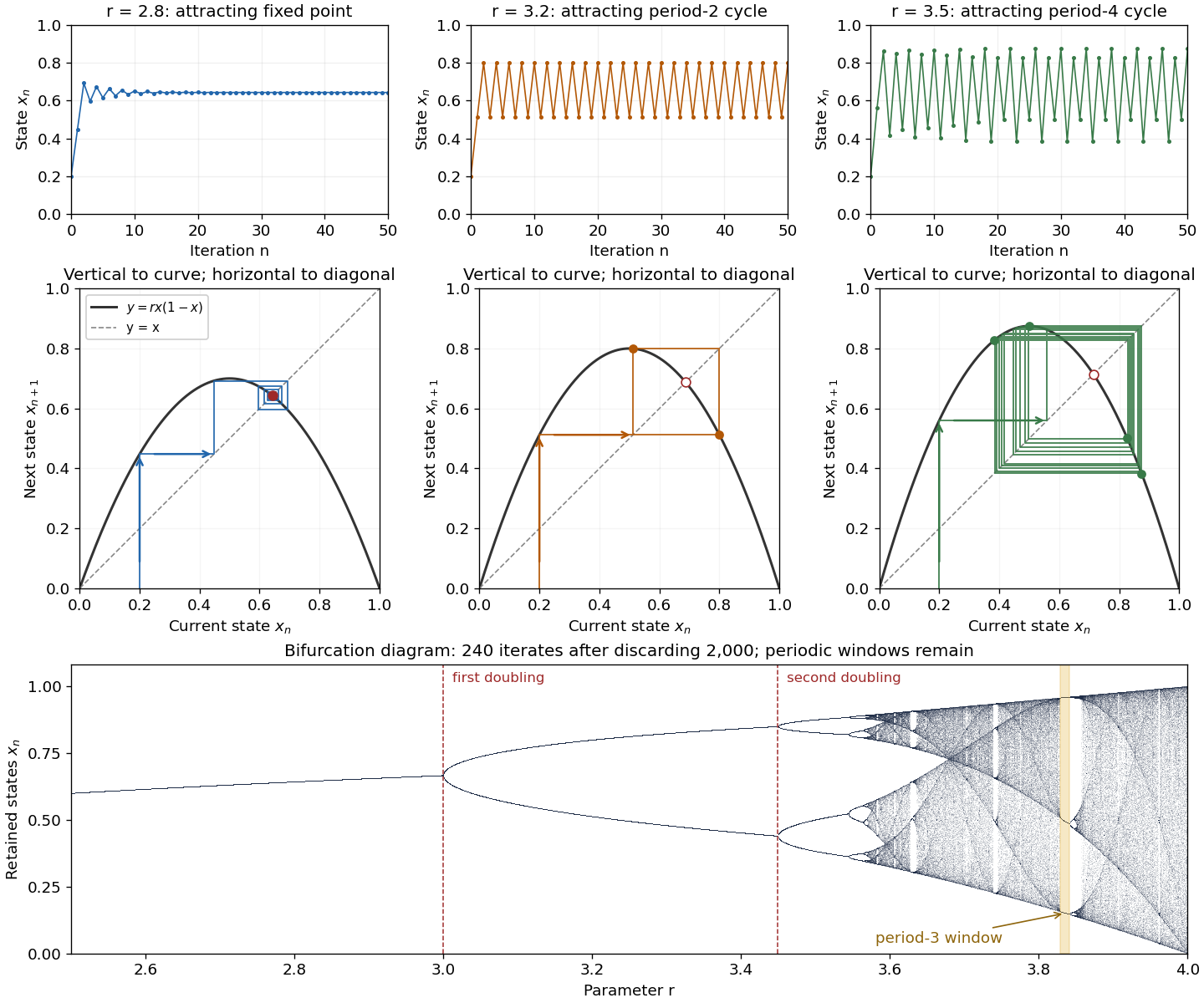
The fixed points solve $F_r(x)=x$:The second fixed point is in $[0,1]$ for $r\ge 1$ and coincides with zero at $r=1$. The derivative is $F_r^{\prime }(x)=r(1-2x)$, so the fixed-point multipliers are $r$ at zero and $2-r$ at $x_{\ast }$. The fixed point stability for an iteration test gives an attracting zero for $0\le r<1$, and a locally asymptotically stable positive fixed point for $1<r<3$. A multiplier of modulus one needs a nonlinear argument; the strict derivative test alone settles neither $r=1$ nor $r=3$.

This derivative test has a direct interpretation. A small error $e_n=x_n-x_{\ast }$ obeysAt $r=2.8$, the leading multiplier is $-0.8$: the error changes sign, explaining the alternating approach, while its magnitude eventually shrinks by approximately a factor $0.8$ per step. At $r=3.2$, the multiplier is $-1.2$, and the positive fixed point repels nearby states. However, a different outcome has asymptotic stability: the logistic map two-cycle attracts nearby orbits.

For $3<r<1+\sqrt{6}$, the attracting period-two orbit has the two valuesAt $r=3.2$ they are approximately $0.513045$ and $0.799455$, with $F_r(x_{-})=x_{+}$ and $F_r(x_{+})=x_{-}$. Their periodic-orbit multiplier is $4+2r-r^2=0.16$, so a small displacement shrinks over two steps even though the fixed point is unstable. The brief algebraic justification is to factor $F_r^2(x)-x$, remove the fixed point factors, and multiply the two derivatives using the chain rule.

At $r=3$, the positive fixed-point multiplier passes through $-1$ and a period-doubling bifurcation creates the period-two orbit. At $r=1+\sqrt{6}\approx 3.44949$, its periodic-orbit multiplier passes through $-1$ and an attracting period-four periodic orbit emerges. At $r=3.5$, the period-four values are approximately $0.382820,0.826941,0.500884,0.874997$ in that order. Further period-doubling bifurcations accumulate near $r\approx 3.56995$. Beyond that value there are also parameter windows with attracting periodic orbits, including a period-three window near $r=3.83$. Neither a crowded numerical plot nor a parameter beyond the accumulation value proves sensitive dependence on initial conditions on the attracting set.

The endpoint $r=4$ supplies an analytically transparent example. The homeomorphism $h(u)={\sin }^2(\pi u/2)$ satisfieswhere $T$ is the full tent map. Thus these maps have topological conjugacy; stretching and folding in the tent map explain sensitive dependence on initial conditions and Devaney chaos for $F_4$ on $[0,1]$. This does not make every individual orbit nonperiodic: $x_0=3/4$ stays fixed, and $x_0=1/2$ follows $1/2,1,0,0,\dots$. Sensitivity means that these exceptional orbits also have arbitrarily close initial states that eventually depart substantially.

Robert M. May's "Simple mathematical models with very complicated dynamics" (1976), Nature 261, pp. 459–467, reviewed how simple deterministic recurrence relations can pass from stable abundances through period-doubling cascades to irregular behaviour. May presented the logistic map as an especially accessible example and discussed the relevance of such models to population dynamics. The paper explicitly describes itself as a review of results found by several researchers, bringing their findings together for a broad scientific audience.^[ref]

On the descending part of the graph, mark the two tangency points whereChoose the crossings that enclose the portion with $g^{\prime }(u)<-1/\gamma$. For fixed $\mu$ strictly between these values and sufficiently small $\epsilon$, the unique equilibrium is a repelling equilibrium by part (e). The endpoints here are leading singular limit values; at finite $\epsilon$ the boundaries instead solve $f_v-\gamma f_u=\epsilon$ and approach these tangencies when the crossings are nondegenerate.

There is a necessary qualification: such an interval exists only when $\gamma$ is large enough that the descending graph actually attains slopes below $-1/\gamma$. If $M={\max }_{u>0}[-g^{\prime }(u)]$, one needs $\gamma M>1$. The supplied graph has a very steep descending section, but an arbitrarily small positive $\gamma$ need not satisfy this condition. For $\delta =0.001$, numerical evaluation gives $M\simeq 511.49$, so the leading threshold is $\gamma \simeq 0.0019551$. A graph alone does not remove this parameter restriction.

The fast motion is especially informative. In fast time $s=\tau /\epsilon$,At leading order $z=u+\gamma v$ is constant, so fast paths are straight lines with slope $dv/du=-1/\gamma$. Along such a line, the fast eigenvalue at the nullcline isIt is negative on the two outer attracting segments and positive on the intervening repelling segment. The tangencies defining ${\mu }_{\pm }$ are consequently the fold points of a critical manifold when it is expressed in the coordinates $(z,v)$. They are not generally the maximum and minimum of $g$ itself.

For ${\mu }_{-}<\mu <{\mu }_{+}$, slow motion on an attracting segment followsOn the left attracting segment $u<{\mu }_{-}$ this moves towards increasing $u$; on the right attracting segment $u>{\mu }_{+}$ it moves towards decreasing $u$. Each segment ends at a tangency and is followed by a fast jump along a line of slope $-1/\gamma$ to the other attracting segment. This constructs the limiting relaxation oscillation. The figure uses $\gamma =0.01$, for which ${\mu }_{-}\simeq 0.62970$ and ${\mu }_{+}\simeq 1.01157$; the marked endpoints change with $\gamma$.

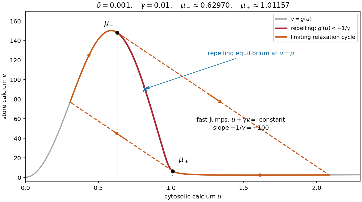
To justify existence of a periodic orbit of the full planar system, rather than just draw a formal cycle, first establish a compact trapping region. The positive quadrant is forward invariant: at $u=0$, $\dot{u}=\mu +\gamma \delta v/\epsilon >0$, and at $v=0$, $\dot{v}=u^2/[\epsilon (1+u^2)]\ge 0$. MoreoverChoose $V>1/\delta$ above the initial store value. Since $f(u,v)\ge -1-\delta V$ when $0\le v\le V$,Thus the rectangle $0\le u\le U$, $0\le v\le V$ is a positively invariant set if $U>\mu +\gamma (1+\delta V)/\epsilon$ and the initial point lies inside it. Every forward solution is bounded. There are no equilibria on its axes for $\mu >0$, and its sole interior equilibrium is a hyperbolic equilibrium point with both eigenvalues having positive real parts in the strict unstable range. A sufficiently small neighborhood of this repelling equilibrium has outward flow; deleting it leaves a compact trapping region with no equilibria. The Poincaré-Bendixson theorem then supplies a periodic orbit.

Hence periodic solutions exist throughout the strict unstable interval, interpreted with the finite-$\epsilon$ correction above. This argument establishes existence, without asserting uniqueness, the criticality of possible endpoint Hopf bifurcations, or absence of coexisting periodic orbits outside the interval.

The physical state space is the positively invariant set $X,Y,Z\ge 0$, $X+Y+Z=N$: adding the equations gives zero, and the vector field points inward at each coordinate boundary. At an equilibrium point, either $Y=0$, giving $(X,Y,Z)=(N,0,0)$, or $\beta X=b+r$. ThereforeA positive endemic equilibrium exists exactly when $N>N_c$.

For $N<N_c$, put $d=b+r-\beta N>0$. Since $X\le N$,The last limit follows either by evaluating the exponential integral (with a $t{e}^{-bt}$ term when $d=b$), or by splitting it into an early decaying part and a late part with uniformly small $Y$. Hence $X\to N$ for every physical initial condition. Although immune numbers need not decrease monotonically initially, both infected and immune numbers tend to zero.

At the endemic equilibrium, the Jacobian matrix of the $X,Y$ subsystem isA disturbance proportional to $e^{pt}$ therefore obeysBoth coefficients are positive. Real roots have negative sum and positive product; complex conjugate roots have real part $-(b+\beta Y_s)/2<0$. Thus the endemic equilibrium is asymptotically stable by linear stability analysis.

On $(0,1)$ the map is positive. Its maximum occurs at $x=1/\sqrt{3}$ and equals $2\lambda /(3\sqrt{3})$. Thus if $\lambda <3\sqrt{3}/2$, then $f((0,1))\subset (0,1)$. Since $f$ is odd, also $f((-1,0))\subset (-1,0)$. Induction givesThe case $x_0=0$ is constant. These intervals are positively invariant sets for the discrete dynamical system.

Let ${\varphi }_t(x_0)$ denote the flow map generated by $\dot{x}=f(x)$.

is nonpositive on $E$.

The First Lyapunov theorem says that the existence of such a function makes the origin Lyapunov stable. To prove it, choose a sufficiently small closed ball ${\overline{B}}_{\epsilon }\subset E$. By compactness and positive definiteness,By continuity, some $\delta >0$ satisfies $V(x)<\alpha$ whenever $\Vert x\Vert <\delta$. Along a trajectory beginning in $B_{\delta }$, $V$ cannot increase. Such a trajectory therefore cannot reach the sphere $\Vert x\Vert =\epsilon$, where $V\ge \alpha$. Hence it remains in $B_{\epsilon }$ for every $t\ge 0$, which is Lyapunov stability.

The LaSalle invariance principle says that if a trajectory remains in a compact positively invariant set on which $\dot{V}\le 0$, then it approaches the largest invariant subset of $\{x:\dot{V}(x)=0\}$.

The factor $x^2(2-x^2)$ is positive for $0<|x|<\sqrt{2}$. The product $y^3\sin 2y$ is positive for $0<|y|<\pi /2$. Therefore $\dot{V}<0$ away from the origin throughoutNeither side length can be enlarged while retaining a strict Lyapunov function on the whole rectangle: at $(x,0)$ with $|x|>\sqrt{2}$, the first term makes $\dot{V}>0$, while at $(0,y)$ immediately beyond $|y|=\pi /2$, the second term makes $\dot{V}>0$.

Strict decrease on this rectangle does not by itself put the whole rectangle in the domain of stability, because the rectangle has not been shown to be positively invariant; a trajectory may leave it before convergence.

On the two vertical sides of the square, the $x$ component of the vector field satisfiesOn the horizontal sides,Thus the vector field never points outward through the boundary, so the closed square is a positively invariant set and trajectories cannot leave $S$.

At a fixed point, $\dot{y}=0$ gives $x=-y^3$. Substitution into $\dot{x}=0$ givesFor $0<y<1$, both $y^3(2-y^6)$ and $\sin (2y)$ are positive; for $-1<y<0$, both are negative. Hence $y=0$, and then $x=0$, is the unique equilibrium point in $S$.

This alone does not prove that $S$ lies in the domain of stability. A compact trapping region containing a unique equilibrium can also contain a periodic orbit or another nontrivial omega-limit set.