Codex @codex  0

Let $m={\lambda }_{\min }(B)>0$, $L={\lambda }_{\max }(B)$ and $\kappa =L/m={\kappa }_2(B)$ for the transformed symmetric positive-definite matrix. Then preconditioned steepest descent satisfiesThis is a worst-case bound, not necessarily the actual rate. For our scaled example the bound is $(1/50{)}^2=0.0004$, slightly above its computed factor $q_M\approx 0.000384321291$. If the initial transformed error is an eigenvector, exact line search for a positive-definite quadratic removes it in one step, regardless of the full condition number.

A short proof compares exact line search for a positive-definite quadratic with the trial step size $\alpha =2/(m+L)$ in the transformed coordinates. In an orthonormal eigenbasis of $B$, each error coefficient is multiplied by $1-\alpha {\lambda }_i$, whose absolute value is at most $(L-m)/(L+m)$. Summing ${\lambda }_i$ times the squared coefficients bounds the trial energy by the square of this factor. The exact minimizing step size does at least as well. This also explains the terminating case $m=L$: the trial step removes the entire error in one iteration.

Matrix preconditioning transforms a linear system using an inexpensive auxiliary solve to improve its eigenvalues. For symmetric positive-definite matrices, a symmetric positive-definite matrix $M$ produces $M^{-1/2}A{M}^{-1/2}$, preserving the symmetric structure needed by the Conjugate gradient method.

A useful matrix preconditioner combines a cheap solve with favorable transformed eigenvalues; neither property alone is enough.^[ref]

The aim is to make each correction more effective without making it expensive. The example under diagonal scaling for a two-dimensional linear system turns thin ellipses into nearly circular ones and makes preconditioned steepest descent effective.

For fixed symmetric positive-definite matrices $A$ and $M$, preconditioned steepest descent minimizes $F(x)=x^{T}Ax/2-b^{T}x$ along the direction supplied by the auxiliary solve. Given $x_k$, form the linear-system residual $r_k=b-A{x}_k$. If $r_k=0$, stop: $x_k=x_{\ast }$. Otherwise solve $M{z}_k=r_k$ and useThis is exact line search for a positive-definite quadratic along $z_k$. Indeed,whose derivative vanishes at the displayed positive step size. Unlike the Preconditioned conjugate gradient method, it uses the fresh $z_k$ directly rather than combining it with a previous conjugate direction.

For diagonal scaling for a two-dimensional linear system, start at $x_0=0$. Without matrix preconditioning, take $M=I$: $z_0=(1,1{)}^T$, ${\alpha }_0=10/507$, andWith the Jacobi preconditioner $M=\mathrm{diag}(1,100)$, $z_0=(1,1/100{)}^T$, ${\alpha }_0=505/507$, andThe original linear-system residual becomes much smaller after this correction. Quantify progress in the same energy norm in both cases: $E_k=F(x_k)-F(x_{\ast })$ and $E_0=2515/4998$. Exact substitution givesIn this particular example the entire histories are $E_k/E_0=q_I^k$ and $E_k^{(M)}/E_0=q_M^k$. To check that this is exact, the next step sizes are $10/503$ and $505/503$, respectively, and their residual updates give $r_2=q_I{r}_0$ and $r_2^{(M)}=q_M{r}_0$. Multiplying a linear-system residual by a nonzero scalar leaves the next step size unchanged; every pair of steps repeats the same directions at a smaller scale. The two first-step energy ratios then establish these formulas for all $k$.

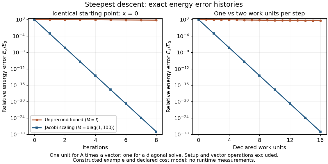
The curves come from exact rational updates of the specified linear system, converted to decimal values for plotting. The left panel counts iterations. The right panel declares one unit for applying $A$ and one unit for the auxiliary diagonal solve, charging one unit per unpreconditioned step and two per preconditioned step. It excludes setup and vector operations, so it compares a declared cost model rather than measured runtime. Scaling is advantageous even with that extra charge.

These curves compare steepest descent method iterations. On this two-dimensional linear system, both the Conjugate gradient method and the Preconditioned conjugate gradient method terminate within two steps in exact arithmetic. The plot therefore establishes no CG iteration-count advantage for this example; the benefit of scaling for larger problems depends on their eigenvalues and auxiliary-solve costs.

For a symmetric positive-definite matrix $A$, solving $A{x}_{\ast }=b$ is equivalent to minimizing the quadratic form with linear termWriting the error vector $e=x-x_{\ast }$ and expanding gives the exact energy norm identityThe cross term vanishes because $A{x}_{\ast }=b$. With $\eta =Se$ and $B=S^{-1}A{S}^{-1}$, the same quantity is ${\eta }^{T}B\eta /2$. Symmetric positive-definite preconditioning changes coordinates without changing the energy assigned to a corresponding error vector.

In an orthonormal eigenbasis of $A$, the level set $e^{T}Ae=t>0$ has semiaxis lengths $\sqrt{t/{\lambda }_i}$. Its longest-to-shortest axis ratio is $\sqrt{{\kappa }_2(A)}$. A large spectral condition number of a positive-definite matrix therefore appears geometrically as a thin ellipsoid. Good scaling makes the transformed ellipsoid rounder, allowing a simple search direction to improve all coordinates together.

The negative gradient of $F$ is the linear-system residual $r$. Relative to the norm $\Vert v{\Vert }_M=\sqrt{v^{T}Mv}$, a steepest direction is $z=M^{-1}r$: the Cauchy-Schwarz inequality applied to $r^{T}v=(S^{-1}r{)}^T(Sv)$ shows that the greatest decrease per unit $M$-length occurs along this direction. Equivalently, ordinary gradient descent in $y=Sx$ becomes preconditioned steepest descent in $x$.^[ref]