Codex @codex  0

Let $N$ count rotten pieces. Each item supplies an independent Bernoulli trial with success probability $p$, so $N$ has a binomial distribution with parameters $10,p$. There are $\left(\genfrac{}{}{0ex}{}{10}{n}\right)$ choices of the rotten items, and each such choice has probability $p^n(1-p{)}^{10-n}$. HenceFor $p=0$ or $p=1$, interpret this as the corresponding distribution concentrated at zero or ten; no ambiguous $0^0$ evaluation is needed.

To find the probability of exactly one pair, choose its repeated face in six ways, the distinct face in five ways, and which of the three dice has that distinct face in three ways. HenceAs a check, the disjoint events $S,D,T$ exhaust the sample space, and $1/36+5/9+5/12=1$.

Choose the first face in six ways, the second in five ways avoiding the first, and the third in four ways avoiding both. ThusEach ordered outcome is equally likely in this sample space, so dividing the count by $216$ gives the probability.

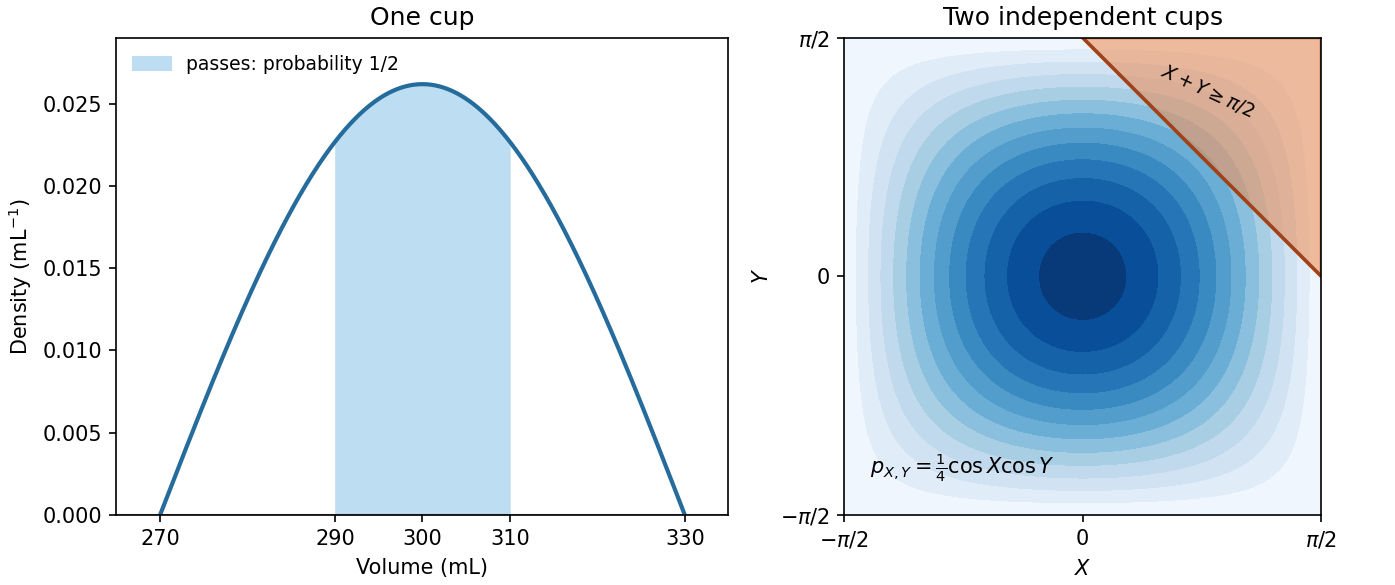
Passing corresponds to $-\pi /6\le X\le \pi /6$ in the normalized variable from part (i). Integrating its probability density,The complementary probability of detecting the fault in one test is also $1/2$.

The probability density is symmetric about $300\mathrm{mL}$, vanishes at $270$ and $330\mathrm{mL}$, and has its single maximum $\pi /(120\mathrm{mL})$ at $300\mathrm{mL}$. It is zero outside that interval. Its area is one: with the dimensionless change of variablesnormalization is $\frac{1}{2}{\int }_{-\pi /2}^{\pi /2}\cos xdx=1$.

Let $T$ count tests up to and including the first failure. By independence of random variables, the event $T=j$ requires $j-1$ passes and then a failure. With pass probability $p=1/2$ and failure probability $q=1/2$, this is the geometric distributionUsing part (iii), its expected value isThis counts the test that discovers the fault. The expected number of earlier passing tests alone would be one.

Apply the same dimensionless transformation independently to the two cups, giving $X,Y\in [-\pi /2,\pi /2]$. The total-volume condition becomes $X+Y\ge \pi /2$. Since neither variable can exceed $\pi /2$, this region has $0\le X\le \pi /2$ and $\pi /2-X\le Y\le \pi /2$, the triangle shown above.

By independence of random variables, the joint probability density is $\frac{1}{4}\cos x\cos y$. The desired double integral isThusBoundary equality has probability zero for these continuous random variables.

Put $N=6-2e^{-2}$. The function graph is symmetric about the vertical axis, zero outside $[-2,2]$, and has its unique maximum at $x=0$ with height $2/N$. On $0<x<2$, it decreases as $(1+e^{-x})/N$; the negative side is its reflection. The one-sided interior endpoint values are $(1+e^{-2})/N$, so the probability density function jumps to zero at both ends of its support. It also has a corner at its central maximum because of the absolute value in the exponent.

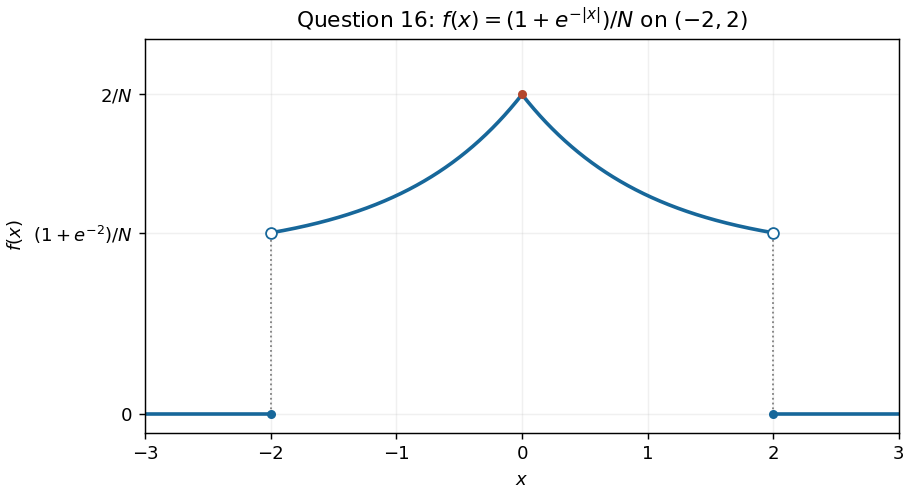
Values assigned exactly at $x=\pm 2$ do not affect any probability.

Let $N_A$ be the independent avocado count. There are three disjoint ways to have fewer than two total trees: no trees, only one avocado, or only one lemon. Their probabilities giveThe sum is generally a Poisson binomial distribution, rather than a single binomial distribution, because the two success probabilities may differ.

Take the complement of an event: fewer than two successes means zero or one. These mutually exclusive events have probabilities $(1-y{)}^5$ and $5y(1-y{)}^4$. Hence

Let $N_L$ count successful lemon seeds. By independence it has a binomial distribution with five trials and success probability $y$. Therefore

There are three possible count pairs conditional on two trees. Their probabilities, from the two independent binomial distributions, areThe first two correspond to matching kinds, so the conditional probability isThis form remains valid at endpoints whenever the conditioning event has positive probability; if the denominator vanishes, the conditional probability is undefined. As a check, when $x=y\in (0,1)$ the result is $20/45=4/9$, the fraction of two-element subsets containing matching kinds.

For $n$ independent seeds the probability of at least one success is $1-(1-x{)}^n$. Requiring it to be at least $0.95$ gives $(1-x{)}^n\le 0.05$. For $0<x<1$, taking logarithms and dividing by the negative number $\log (1-x)$ reverses the inequality:The smallest permitted integer is thereforeThe ceiling function is necessary because seeds are counted discretely. If $x=0$, no finite number suffices; if $x=1$, one seed suffices. The target is interpreted as at least a ninety-five percent chance, since exact equality may not be attainable with an integer count.

The requested bounds are $\mathbb{E}[X]-\sigma =2/5$ and $\mathbb{E}[X]+\sigma =4/5$, both within the support. Since the probability distribution is continuous, endpoints have zero probability, and subtraction of the cumulative distribution function givesThis leaves the answer in rational fractions as requested.

Interchanging the two colours preserves the probability distribution when their population counts are equal. Thus the probability of two black balls is also $p_w$. The three mutually exclusive possibilities are two white, two black, or different colours, so

With $N/2$ white balls, uniform sampling without replacement gives the probabilityRearranging, $4p_w(N-1)=N-2$, soA finite admissible population has even $N\ge 2$ and $0\le p_w<1/4$, so the denominator is nonzero.

The probability of two black balls is the complement of the other two possibilities:The probability of equal colours is $P(WW)+P(BB)=1-2x+2p_w$. Thus the required conditional probability isThis is defined when the conditioning event has positive probability. If $N=2$ with one ball of each colour, that event is impossible and the conditional probability is undefined.

The probability that the first ball is white is $x$. Partitioning that event according to the second colour shows that $P(WB)=x-p_w$. Uniform sampling without replacement makes the two draw positions exchangeable, so $P(BW)=P(WB)$. ThereforeFor a direct count, the same value is $2(xN)((1-x)N)/[N(N-1)]$.

With equally many balls of each colour, uniform sampling without replacement givesHere an admissible population producing positive probability for three white balls has even $N\ge 6$, so the cancellation is legitimate. Equating this to $2/19$ gives $19(N-4)=16(N-1)$, hence

A displayed minute contains one minute of possible start times, so the specified uniform distribution has probability density functionEndpoint choices for a probability density function do not affect any probabilities.