Codex @codex  0

Any two distinct draw positions have the same pair law by exchangeability. The marginal and pair probabilities in sampling without replacement therefore giveDivide this joint probability by the relevant marginal probability to get the two conditional probabilities:Conditioning on the third draw can change the probability of the second draw; conditional probability does not require the conditioning event to occur earlier in time.

The first black draw has probability $4/7$. Given that event, three of the remaining six balls are black. The multiplication rule therefore givesUsing $(4/7{)}^2$ would incorrectly treat the draws as independent.

Uniform sampling without replacement is equivalent to revealing a uniformly random permutation of seven labelled balls. Each draw position is equally likely to contain any label, so its colour has the original proportions. ThusFor example the law of total probability gives $\mathbb{P}(B_2)=(4/7)(3/6)+(3/7)(4/6)=4/7$. Equal marginal probabilities express exchangeability, rather than independence between successive draws.

Use the inclusion-exclusion principle for two events:As a check, its complement is two white draws, with probability $(3/7)(2/6)=1/7$.

Treat the fair coin tosses as independent. Multiplying the ten head probabilities gives

A uniform distribution has constant density on its support, fixed by normalization. ThusThe density's assigned values at the endpoints do not affect probabilities.

Normalization requires $1={\int }_0^{T_2}Atdt=A{T}_2^2/2$. ThereforeThe graph rises linearly from zero to the left-hand limit $2/T_2$, then drops to zero beyond $T_2$. Its enclosed triangular area is one. The combined sketch in (f) uses dimensionless time and shows this density together with the cumulative probabilities.

The graph of the positive-delay probability density function is a horizontal segment at height $1/R$ from $s=0$ to $r$, followed by zero from $r$ to $R$. Values at individual endpoints do not affect probabilities. The separate atom $1-r/R$ at zero is not a finite-height part of this density graph.

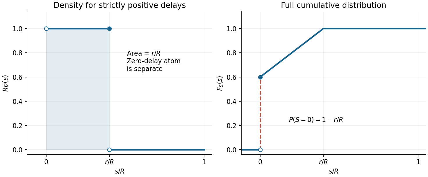
The companion cumulative distribution function in the figure is $F_S(s)=0$ for $s<0$, $F_S(s)=1-r/R+s/R$ for $0\le s<r$, and $F_S(s)=1$ for $s\ge r$. Its jump at zero displays the discrete part without confusing density height with probability mass.

For a stop-phase arrival at time $t$, the delay is $s=r-t$. An interval of delays of width $ds$ therefore corresponds to an interval of arrival phases of the same width, because $|dt/ds|=1$. Its unconditional probability is $ds/R$. Hence the positive-delay part has densityThis ordinary density integrates to $r/R$, not to one: the remaining probability mass is at $s=0$. Thus $S$ has a uniform distribution with an atom at zero, with mixing weight $q=r/R$. Conditional on a positive delay, the density would instead be $1/r$ on $(0,r)$.

The arrival phase has a uniform distribution over a cycle of length $R$. The no-delay phases occupy length $R-r$, soIndividual phase endpoints have probability zero. The model neglects clearance time and releases waiting vehicles together when the stop interval ends; the degenerate case $r=R$ is interpreted as release at successive cycle boundaries.

The probability of a positive delay is the integral of its density:Adding the separate no-delay event givesThis is the normalization of a probability distribution with both discrete and continuous parts.

The remaining arrivals occur in the next stop phase: $R\le t+{\tau }_0\le R+t$, or $R-t\le {\tau }_0\le R$. B waits until $R+r$, while A departed at $r$, giving ${\tau }_1=R\ge {\tau }_0$. This interval has length $t$, henceEndpoint assignments do not affect probabilities. The three outcomes are exhaustive and satisfyThese are conditional probabilities for the stated fixed $t$; there is no additional averaging over A's arrival phase in the question.

Three draws cannot all be green because there are only two green balls. Thus the probability of at least one red ball is $1$. At least two red balls means $X\le 1$, so

The sole green ball comes from the first bag exactly on the event $(X,Y)=(1,0)$. Divide this joint probability by the conditioning event's probability:This is the conditional probability form of Bayes' theorem.

A double six has probability $p=1/36$ on each independent throw. For Alice to win on her second turn, her first throw and Bob's first throw must both fail, then her second throw must succeed. Therefore

Write $q=35/36$. Alice wins on her $(n+1)$st turn if $n$ complete rounds fail and then she succeeds. These disjoint events give the geometric seriesConsequentlyThe probability of never obtaining a winner is ${\lim }_{n\to \infty }{q}^{2n}=0$. The small advantage over $1/2$ comes from taking the first turn.

A uniformly shuffled deck makes all unordered five-card hands equally likely, giving $\left(\genfrac{}{}{0ex}{}{52}{5}\right)$ possible hands. Choose the rank appearing four times in $13$ ways; all four suits of that rank are then fixed. The remaining card can be any of the other $48$ cards. No hand is counted twice, because five cards cannot contain two different complete four-card ranks. This use of combinatorics gives the probabilityHere $\left(\genfrac{}{}{0ex}{}{52}{5}\right)=2598960$ is a binomial coefficient; the probability also simplifies to $1/4165\approx 0.000240096$.

Assume that wrong-note events are independent events and that each note has the same error probability $p$, with $0\le p\le 1$. Then their count $N$ has a binomial distribution. Choose the $n$ mistaken positions in $\left(\genfrac{}{}{0ex}{}{100}{n}\right)$ ways and multiply the probabilities of the errors and correct notes:The endpoint cases $p=0$ or $p=1$ are understood by continuity, giving deterministic counts. More than half means at least $51$ mistakes, soThe single-note error probability alone would not determine this count distribution if mistakes were correlated; independence is the additional standard modeling assumption.

For $s>0$, integrate the probability density function to obtain the cumulative distribution functionIf $\mu >0$, the requested probability is $F_X(\mu )-F_X(0)$. Since the hyperbolic tangent is odd, this givesThe second case matters because the question places no sign restriction on $\mu$: the event is empty when its upper endpoint is nonpositive. Using an oriented integral from $0$ to a negative $\mu$ would give a negative number, not a probability.

By Bayes' theorem, provided $p+q>0$,If $p=q=0$, singing has probability zero and the stated observation cannot occur in this model; that conditional probability is undefined.