Codex @codex  0

Bayes' theorem updates a hypothesis using observed data. For mutually exclusive exhaustive hypotheses $H_j$ and data $D$ of nonzero probability,The prior $P(H_j)$ describes information before these data; the likelihood $P(D\mid H_j)$ describes the sampling model; the denominator is the evidence; and the posterior is the updated probability. likelihood and posterior are different conditional quantities. For a continuous parameter, sums become integrals and the posterior is a probability density.

Consider a counter registering independent events at unknown constant rate $\lambda$, observed for known exposure $T$ with negligible background and dead time. The observed count has a Poisson distribution:Take a proper gamma prior in shape-rate convention,Multiplying by the likelihood adds the count to the shape and the exposure to the rate. Normalization therefore givesHere $\beta$ has exposure units. This is Poisson-gamma conjugacy. Successive independent counting runs update the same posterior by adding their counts and exposures, so the result agrees with analysing all the data together.

A credible interval contains a specified posterior probability for $\lambda$, conditional on the chosen prior and model. For low counts, the posterior can be asymmetric and sensitive to the prior, and a symmetric Gaussian error bar can be misleading. For large $n$ and an exposure dominating prior information, the mean approaches $n/T$ and its standard deviation approaches $\sqrt{n}/T$. Background, missed events or time-dependent rates require a richer likelihood; Bayes' theorem cannot compensate for an incorrect physical counting model. The prior must be specified independently of the same data being used in the likelihood, unless its estimation is explicitly included in a larger model.

Reduced radial equation. A spherical harmonic satisfies ${\hat{L}}^2{Y}_{\ell m}=\ell (\ell +1){\hslash }^2{Y}_{\ell m}$. Substitute $\psi =R{Y}_{\ell m}$ into the time-independent Schrödinger equation, divide out the angular function, and put $R=U/r$. Direct differentiation givesMultiplication by $r$ then gives the Radial Schrodinger equationHere $\mu =m_1{m}_2/(m_1+m_2)$ is the reduced mass, and the extra positive term is the centrifugal potential.

Boundary conditions. At the origin this finite central potential has no point interaction. The physical radial solution is regular there, requiring $U(0)=0$; for $\ell =0$, a nonzero constant $U(0)$ would give $R\sim 1/r$ and a point-source singularity of the three-dimensional Laplacian. Mere square integrability alone would not remove that singular solution. For a bound state, the radial probability integral is ${\int }_0^{\infty }|U{|}^{2}dr$, so the exterior solution must decay and $U(r)\to 0$ as $r\to \infty$.

Solutions for zero orbital angular momentum. For $\ell =0$ and $-V_0<E<0$, defineThe interior equation is $U^{\prime \prime }+k^{2}U=0$; $U(0)=0$ excludes the cosine. The exterior equation is $U^{\prime \prime }-q^{2}U=0$; normalizability excludes the growing exponential. ThusThe constants cannot remain independent once the interface is matched. Since the potential step is finite, both $U$ and $U^{\prime }$ are continuous at $a$:Dividing the equations yields

Existence and number of s-wave bound states. Put $z=ka$, $y=qa$, and ${\rho }_0=a\sqrt{2\mu V_0}/\hslash$. ThenThe lowest branch lies on $\pi /2<z<\pi$. Along it, $y=-z\cot z>0$ and ${\rho }_0=z/\sin z$ increases continuously from $\pi /2$ to infinity. Therefore a first negative-energy solution exists precisely when ${\rho }_0>\pi /2$, orFurther branches begin at $z=3\pi /2,5\pi /2,\dots$ as $q\to 0^{+}$. Hence the bound-state thresholds of a spherical square well give exactly one negative-energy $\ell =0$ state whenThe upper equality is included: the second branch is then only at $E=0$, with constant exterior $U$, and is not normalizable. If threshold cases are excluded by convention, the commonly quoted open interval has a strict upper inequality; the physical negative-energy state count at equality is still one.

Deuteron estimate. Using $m_p{c}^2\simeq 938.27\mathrm{MeV}$, $m_n{c}^2\simeq 939.57\mathrm{MeV}$ and $\hslash c\simeq 197.327\mathrm{MeV}\mathrm{fm}$ gives $\mu c^2\simeq 469.46\mathrm{MeV}$. At $a=2.1\mathrm{fm}$,The threshold for a second $s$ state is $9V_{\ast }\simeq 209\mathrm{MeV}$, far above the stipulated depth $33.5\mathrm{MeV}$. Thus this model has no radially excited s-wave bound state.

Checking other orbital angular momentum sectors matters before ruling out every excitation. At the first $p$-wave threshold, the regular interior reduced radial function is $r{j}_1(kr)$ and the zero-energy exterior function is proportional to $r^{-1}$. Matching their logarithmic derivatives requires $j_0(ka)=0$, whose first root is $ka=\pi$. HenceLarger $\ell$ only increases the centrifugal potential. Therefore no bound orbital excited states are expected in the specified central square-well model. Its spin dependence and tensor nuclear forces have not been specified; the calculation does not resolve the real deuteron's internal spin structure.

Distinguishable noninteracting particles. Interpret $V$ as the same external one-particle potential for each particle; the total potential is $V({\mathbf{r}}_1)+V({\mathbf{r}}_2)$. The Time-dependent Schrödinger equation isLet $\hat{h}{\varphi }_a={ϵ}_a{\varphi }_a$ and $\hat{h}{\varphi }_b={ϵ}_b{\varphi }_b$, where $\hat{h}=-{\hslash }^2{\nabla }^2/(2m)+V$. Applying ${\hat{h}}_1+{\hat{h}}_2$ to the product multiplies it by ${ϵ}_a+{ϵ}_b$. The time derivative of $e^{-iEt/\hslash }$ multiplies it by $E$. Thus the proposed stationary product is a solution providedThe tensor product separates the two independent one-particle dynamics.

Identical spin-one-half particles. Identical fermions require antisymmetry under exchange of the complete position-and-spin labels. First take $a,b$ to be distinct orthonormal spatial orbitals, and defineThe symmetric spatial state must multiply the antisymmetric spin-one-half singlet state; the antisymmetric spatial state must multiply one of the three symmetric spin-one-half triplet states. The four normalized possibilities, each with the common time factor $e^{-iEt/\hslash }$, areThese are the required product states under fermionic exchange symmetry. If $a=b$, the antisymmetric spatial combination vanishes. Only the product ${\varphi }_a({\mathbf{r}}_1){\varphi }_a({\mathbf{r}}_2)$ times the singlet remains, as required by the Pauli exclusion principle. A nonorthogonal pair would require different normalization factors; the displayed $1/\sqrt{2}$ assumes an orthonormal stationary-state basis.

Weak repulsive Coulomb interaction. For fixed orbitals $a,b$, first-order perturbation theory gives spatial energy shifts $J\pm K$. Here $J$ is the direct interaction energy, while the exchange integral for repulsion strength $g>0$ isThe positivity follows from the positive Fourier transform of the Coulomb kernel. Consequently Coulomb exchange splitting of two orbitals givesAll three triplet spin components remain degenerate for a spin-independent Coulomb interaction. Their antisymmetric spatial factor vanishes at coincidence and reduces close encounters. The inequality is strict when $K>0$; for negligible orbital overlap, the splitting may vanish. This comparison fixes one particle in each of the specified orbitals and does not rank singlets with a different orbital occupation.

Spin-zero bosons. For one particle in each of the same distinct orthonormal orbitals, the spin factor is symmetric and bosonic exchange symmetry requires ${\Phi }_{+}$. At coincident positions,Thus the bosonic coincidence enhancement in two orthogonal orbitals isThese are joint probability densities, or small-detector-volume limits; an exactly specified point has zero probability in a continuous distribution. If both particles occupy the same orbital, the properly normalized product is already symmetric and the corresponding enhancement relative to distinguishable particles in that same orbital is one. The paper's usual factor-two answer presumes distinct orthogonal input orbitals.

A Hermitian operator satisfies the adjoint symmetry conditionfor vectors in its specified domain. For a finite matrix this means $A=A^{†}$. For an unbounded differential operator, boundary conditions and domains matter: symmetry on a chosen domain is not alone sufficient for self-adjointness. Physical observables require the corresponding self-adjoint operator and its spectral measure. This distinction prevents purely formal integration by parts from being mistaken for a complete operator definition.

Real eigenvalues. If $A|a⟩=a|a⟩$ with nonzero norm, Hermiticity impliesso $a=a^{\ast }$. Thus eigenvalues representing measurement outcomes are real.

Orthogonality. For eigenvectors $|a⟩,|b⟩$,Hence $(a-b)⟨b|a⟩=0$, and distinct eigenvalues have orthogonal eigenvectors. Within a degenerate eigenspace, Gram-Schmidt orthogonalization can choose an orthonormal basis. In finite dimensions the spectral theorem gives a complete orthonormal eigenbasis andwhere $P_a$ projects onto each eigenspace. In infinite dimensions a continuous spectrum may require a spectral integral rather than a normalizable eigenvector for every possible outcome; a position operator on the full line is a familiar example.

Measurements and probabilities. In the discrete case the Born rule assigns probability $⟨\psi |P_a|\psi ⟩$ to the outcome $a$. For a nondegenerate eigenbasis, $|\psi ⟩={\sum }_a{c}_a|a⟩$ gives probabilities $|c_a{|}^2$, withThe variance vanishes precisely when the state lies in an eigenspace with a single sharp outcome. A repeatable ideal projective measurement prepares the corresponding eigenspace; superpositions of different eigenvalues do not have a preassigned sharp value of that observable in this description.

Compatibility and dynamics. Commuting Hermitian matrices admit simultaneous diagonalization, permitting a common set of sharp labels. For example $L^2,L_z$ commute, whereas $L_x,L_y$ do not. In the differential-operator setting the corresponding spectral compatibility requires appropriate domain conditions. Noncommuting observables obey the Robertson uncertainty principleThe canonical commutation relation then gives $\Delta x\Delta p\ge \hslash /2$.

The Hamiltonian operator represents energy. A self-adjoint $H$ generates unitary time evolution, $U(t)=e^{-iHt/\hslash }$, preserving norm and total probability; its eigenvalues determine stationary-state phases and transition energies. Hermiticity supplies real outcomes and orthogonal eigenspaces, while self-adjointness and the spectral theorem make these measurement and evolution rules mathematically complete.

A Gaussian distribution with mean $\mu$ and standard deviation $\sigma$ has probability densityIts symmetry, finite variance and simple behavior under linear combinations make it useful for repeated measurements. Roughly $68.3\%$, $95.4\%$ and $99.7\%$ of observations lie within one, two and three true standard deviations of the mean. These are coverage probabilities for a specified distribution, not guarantees that every experimental error is normal.

Why it appears. The central limit theorem explains why many sums of small independent finite-variance contributions approach a Gaussian law after centering and scaling, provided no single contribution dominates. Detector noise, small mechanical disturbances and multiple electronic fluctuations can combine approximately this way. The theorem does not remove a common calibration bias, and it does not justify assuming normal tails for rare large disturbances or arbitrarily correlated errors. A large-mean Poisson distribution also approaches a Gaussian with variance equal to its mean, making normal approximations useful for high-count photon or particle data; low counts require the discrete model.

A classical particle at thermal equilibrium in a one-dimensional harmonic potential has a Gaussian position distribution directly from the Boltzmann distribution:Thus a Gaussian law can arise from the energy dependence of equilibrium probability, rather than only from an informal appeal to many independent errors.

Precision of repeated measurements. For $N$ independent observations with the same mean and variance, the sample mean has variance ${\sigma }^2/N$. For Gaussian observations this mean is exactly Gaussian:Consequently quadrupling the number of independent readings halves the random standard error. When the true variance is unknown, a small-sample confidence interval for a normal mean uses a Student t-distribution with $N-1$ statistical degrees of freedom; replacing that by a normal quantile can overstate precision. Shared systematic errors and correlations do not decrease by the same averaging rule.

Combining results and fitting models. Independent Gaussian estimates $x_i$ of one quantity, with known variances ${\sigma }_i^2$, combine through the inverse-variance weighted meanFor a model $y_i=g_i(\theta )+{ϵ}_i$ with independent zero-mean Gaussian noise, maximizing the likelihood is equivalent to minimizing the weighted least-squares statisticFor a correct linear model with known independent Gaussian errors and $p$ fitted parameters of full rank, the minimized statistic has a chi-squared distribution with $N-p$ degrees of freedom. Nonlinear fits only inherit that familiar approximation under additional regularity and adequate-data assumptions. Known correlated Gaussian errors require the full inverse covariance matrix in the quadratic form.

These properties support confidence intervals, consistency checks, calibration and error propagation. They also give practical diagnostics: inspect residuals for trends, changing spread, correlations or outliers before trusting a Gaussian fit. Gaussian models connect physical fluctuations to quantitative uncertainty, but their assumptions must be checked rather than inferred from the shape of a convenient bell curve.

Let $\rho ={\psi }^{\ast }\psi$ be the probability density. For a real potential energy $V(x)$, the Schrödinger equation and its complex conjugate areDifferentiate $\rho$ and substitute both equations. The potential terms cancel, leavingComparison with the probability continuity equation ${\partial }_t\rho +{\partial }_{x}J=0$ identifiesFor a plane wave of amplitude $A$ and positive wavenumber $k$, $J=\hslash k|A{|}^2/m$, the density times the velocity. Integrating the continuity equation over an interval makes its probability change equal to the incoming current minus the outgoing current.

SetAll are real and $k_0>k_1>k_2>0$. Suppressing a common time quantum phase $e^{-iEt/\hslash }$, chooseThe rightmost region has no left-moving term because no wave is incident from the right. The shifted quantum phase convention makes $F$ the transmitted amplitude at the second interface.

For finite potential steps and equal mass, wavefunction matching at a finite potential step requires continuity of both $\psi$ and ${\partial }_x\psi$. Explicitly,A discontinuous wavefunction would introduce an inadmissible singular kinetic term, while integrating the stationary Schrödinger equation across a finite step shows that the derivative cannot jump. These conditions also keep the probability current continuous, so a finite interface neither creates nor destroys probability. The derivative rule would need modification for a delta-function potential or a different effective mass; neither occurs here.

The infinite wall imposes $\boxed{\Psi (0)=0}$, and the wavefunction vanishes for $x<0$. The even full-oscillator ground state fails this boundary condition; the lowest admissible state is the positive-half restriction of the odd first excited state. Multiplying by $\sqrt{2}$ restores normalization because half its probability originally lay on either side.

With $\ell =\sqrt{\hslash /(m\omega )}$, the half-harmonic oscillator ground state isIt rises from zero at the wall, reaches its wave-amplitude maximum at $x=\ell$, and decays to zero as $x\to \infty$. It is positive throughout the interior of the allowed region, with no interior node, as required for its ground state. The wall need not make the derivative continuous with the forbidden half-line.

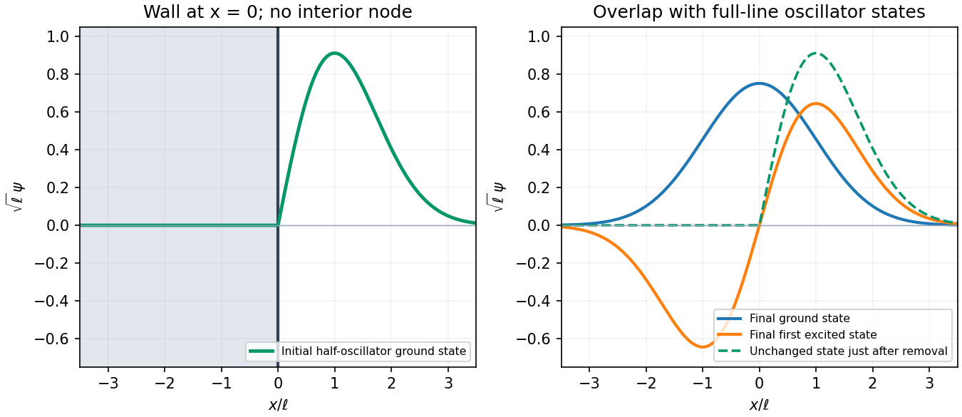
For removal of a half-oscillator wall, the sudden approximation keeps the state unchanged during the change of potential. Its probability in the new full-oscillator ground state ${\Psi }_0={\pi }^{-1/4}{\ell }^{-1/2}{e}^{-x^2/(2{\ell }^2)}$ is the squared overlap:where ${\int }_0^{\infty }x{e}^{-x^2/{\ell }^2}dx={\ell }^2/2$. ThereforeThe integral runs only over the initially occupied half-line. The initial state is not the odd full-line eigenstate: it is zero, rather than negative, on the left. Indeed its overlap with that final first excited state is $1/\sqrt{2}$, giving probability $1/2$, and the remaining probability lies in higher states. Subsequent evolution under the new fixed Hamiltonian operator changes the quantum phases of its energy components without changing these energy-measurement probabilities.

The postulates of quantum mechanics give a framework for predicting observations from a prepared state. The experiments below motivate different features of that framework; no one experiment proves the whole set of postulates or specifies every Hamiltonian operator.

A pure quantum state is a normalized vector in a complex Hilbert space, with vectors differing by an overall quantum phase representing the same physical preparation. In position representation, $\int |\psi (\mathbf{r}){|}^2{d}^{3}r=1$. The linear state space permits quantum superposition, while the Born rule assigns probability ${\int }_{\Omega }|\psi {|}^2{d}^{3}r$ to a position outcome in a region $\Omega$. The wavefunction is a probability amplitude; it is not a classical distribution of definite particle positions and momenta.

An observable is represented by a self-adjoint operator. If $Q$ has spectral projectors $P_q$, its possible measurement outcomes are its spectral values and $\mathrm{Pr}(q)=⟨\psi |P_q|\psi ⟩$. The mean is $⟨Q⟩=⟨\psi |Q|\psi ⟩$. For an ideal repeatable projective measurement, obtaining $q$ leaves the normalized conditional state $P_q\psi /\sqrt{\mathrm{Pr}(q)}$. This projects onto an entire eigenspace if the outcome is degenerate. General detectors need more general measurement in quantum mechanics models; the projective update is an idealization. Noncommuting observables need not have simultaneous sharp values, as the canonical commutation relation and Heisenberg uncertainty relation illustrate.

Between measurements, an isolated system has unitary time evolution generated by its Hamiltonian operator:This preserves normalization and superpositions. Composite systems use a tensor product of state spaces, allowing entangled states as well as product states; identical particles additionally require the bosonic or fermionic exchange symmetry appropriate to their species. Statistical mixtures are described by a density matrix, with $\mathrm{Pr}(q)=\mathrm{tr}(\rho P_q)$. These rules separate preparation, coherent evolution and measurement.

The photoelectric effect exposes discrete energy transfer by light. Illuminate a clean metal cathode in an evacuated tube and measure the collected electron current while varying the light frequency, intensity and a retarding voltage. The stopping potential $V_s$ probes the largest emitted electron kinetic energy, whereas the photocurrent measures the rate at which charge is collected. In the ordinary single-photon regime there is a threshold frequency; above it the maximum energy grows with frequency, rather than with intensity. Changing intensity at fixed frequency mainly changes the number of emitted electrons. These observations are summarized by the Einstein photoelectric equationHere $\Phi$ is the surface work function, and the stopping voltage is understood after any photoelectric contact-potential correction. A photon delivers $h\nu$ in an absorption event; emission is allowed only when that energy can pay the escape cost. This accounts for the frequency threshold and the lack of the classical waiting time associated with slowly accumulating energy in a single electron. The experiment supports energy quantization of light; it does not imply that every incident photon emits an electron or that every emitted electron has the maximum energy. Surface losses and collection geometry affect the full current-voltage curve.

The Davisson–Germer experiment demonstrates a complementary wave property of matter. An electron gun uses a heated emitter, accelerating voltage and apertures to send a narrow beam onto a nickel single crystal in vacuum. A movable collector measures scattered electric current versus direction; rotating the crystal also tests its azimuthal symmetry. The crystal gives sharp angular beams whose positions depend on voltage and crystal orientation. A prominent feature occurs near $54\mathrm{V}$ accelerating voltage and roughly $50^{\circ }$ detector colatitude. The nonrelativistic de Broglie wavelength predicted at that voltage isDiffraction wavelengths inferred using the known crystal structure agree with this voltage dependence. These angular peaks arise from coherent addition of scattering amplitudes from the crystal, not from classical specular reflection of independent point projectiles. Bragg's law is $2d\sin {\theta }_B=r\lambda$ for lattice-plane spacing $d$ and angle to those planes; a detector colatitude is a different angle and must not be substituted without its geometry. The historical readout was current, not a photograph of individual electron trajectories.^[ref]

The double-slit experiment makes the role of amplitudes especially direct. A coherent source illuminates two narrow slits; an observation screen a distance $D$ away records the pattern. For slit spacing $d$ and small screen displacement $y$, the path difference is approximately $dy/D$. The two amplitudes add before probabilities are formed:For equal coherent illumination the interference term varies as $\cos (2\pi dy/(\lambda D))$, giving fringe spacing $\lambda D/d$ beneath the single-slit diffraction envelope. Blocking one slit removes that cross term. Young's optical experiment established wave interference; later particle-resolved realizations with photons or electrons show localized detection events whose accumulated distribution has the interference pattern. Low arrival rates demonstrate that this pattern does not require different incident particles to collide with one another.

If the paths become correlated with distinguishable detector states $|D_1⟩$ and $|D_2⟩$, the cross term acquires their overlap $⟨D_2|D_1⟩$. Perfectly distinguishable path records make that overlap zero, suppressing interference even if the spatial beams still overlap. This connects quantum entanglement, measurement and loss of observable coherence. Without a path measurement, the two alternatives are amplitudes for one preparation, rather than classical mutually exclusive events whose probabilities may simply be added.

Together these experiments motivate a description in which energy transfer and detector outcomes can be discrete, yet propagation retains complex quantum phases and interference. The Born rule connects those amplitudes to repeatable frequencies of outcomes. The Schrödinger equation supplies the dynamics once a Hamiltonian operator is specified, while observable operators, state preparation and the measurement model specify what the apparatus can read.

Quantum tunnelling is transmission through a finite classically forbidden region, where $E<V(x)$. The stationary Schrödinger equation permits an evanescent wavefunction inside such a barrier rather than forcing it to vanish at its entrance. Matching to propagating states beyond a barrier of finite width gives a nonzero transmitted probability current.

For a rectangular barrier of height $V_0$ and width $a$, with equal exterior potentials and $0<E<V_0$, write $\kappa =\sqrt{2m(V_0-E)}/\hslash$. The exact rectangular-barrier tunnelling probability isFor an opaque barrier its dominant dependence is $e^{-2\kappa a}$. For a slowly varying barrier, the WKB approximation generalizes this to $T\sim \exp [-(2/\hslash ){\int }_{x_1}^{x_2}\sqrt{2m(V(x)-E)}dx]$, apart from matching prefactors. Barrier width, particle mass and energy therefore have a strong influence. Energy is conserved in a static barrier: tunnelling does not require the particle to borrow energy or acquire a classical path with negative kinetic energy.

In alpha decay, a nuclear alpha-particle configuration is confined by the short-range nuclear interaction but separated from the exterior by a Coulomb barrier. Its energy can be positive relative to infinity while still lying below the barrier maximum. Escape by tunnelling produces alpha particles at that conserved energy, with an exponentially small decay probability per nuclear encounter. The pronounced dependence of half-life on alpha energy is a characteristic consequence of the barrier exponent, unlike a simple classical escape threshold.

In scanning tunneling microscopy, a conducting tip is brought within a nanometer-scale vacuum gap of a conducting surface and biased weakly. Electron tunnelling gives a current that depends approximately exponentially on separation, $I\propto V{e}^{-2\kappa s}$ in a simple low-bias model. Feedback adjusts the tip height to keep current fixed while scanning, producing a surface map sensitive to both geometry and electronic states. Finite current through the non-contact gap, and its steep dependence on separation, are the direct tunnelling signatures; current is not a direct measurement of topographic height alone.

A Josephson junction provides a collective superconducting example. Two superconductors separated by a thin barrier can carry a coherent pair current $I=I_c\sin \phi$ even at zero voltage. At constant voltage the AC Josephson effect gives $d\phi /dt=2eV/\hslash$ and oscillation frequency $2eV/h$. The coupled condensate quantum phases and pair transfer distinguish this from independent normal-electron transmission. These examples involve different microscopic barriers, but all require quantum coupling across a region that suppresses classical passage. Comparing weak-temperature tunnelling behavior with thermally activated escape helps distinguish the mechanisms experimentally.

A chi-squared test compares residuals with the random scatter predicted by a model. For independent measurements $y_i$ with known Gaussian standard deviations ${\sigma }_i$ and predictions ${\mu }_i(\theta )$, formIf the mean model and error assumptions are correct, a full-rank linear fit of $p$ parameters gives a chi-squared distribution with $\nu =N-p$ statistical degrees of freedom. With a fully specified prediction and no fitted parameters, $\nu =N$. Nonlinear fits usually make this an approximation. Independent external calibration is not the same as fitting a parameter to these test data.

Under the reference distribution, the mean statistic is $\nu$ and its variance is $2\nu$. The upper-tail p-value $\mathrm{Pr}({\chi }_{\nu }^2\ge Q_{\mathrm{obs}})$ quantifies how unusual a discrepancy at least this large would be under the assumed model. A small value suggests model failure or incorrect uncertainties; it is not the probability that the model is true. An unusually small statistic can also reveal inflated uncertainties or correlations. A rejection threshold should be specified in advance.

For independent Poisson distribution counts, the model variance is its expected count ${\mu }_i$. The Pearson chi-squared statistic is $\sum (y_i-{\mu }_i{)}^2/{\mu }_i$. The estimated-error alternative ${\sigma }_i\simeq \sqrt{y_i}$ is common for large counts but can differ substantially when counts are small. In that regime the Poisson deviance or a direct likelihood calculation is preferable, with simulation if an accurately calibrated goodness-of-fit probability is required.

Bayes' theorem updates prior knowledge using the likelihood of new observations. For alternative hypotheses $H_j$,The prior $P(H_j)$ describes information before the data $D$; $P(D\mid H_j)$ is the sampling likelihood, and the posterior $P(H_j\mid D)$ describes the updated probabilities. Posterior odds equal prior odds times the likelihood ratio. A likelihood is a probability model for data at specified parameters, not automatically a normalized probability distribution over those parameters.

For a continuous parameter $\theta$, the same rule uses densities: $\pi (\theta \mid D)=L(D\mid \theta )\pi (\theta )/\int L(D\mid u)\pi (u)du$. Priors can encode positivity, physical limits, previous independent measurements or calibration knowledge. Their parameterization matters: a density uniform in a rate is not uniform in its logarithm. Proper priors make model evidences well defined; an arbitrary normalization in an improper prior is especially problematic for comparing models.

A counting example uses Poisson-gamma conjugacy. If a detector registers $K$ events in exposure $t$ with constant rate $\lambda$, $L\propto {\lambda }^K{e}^{-t\lambda }$. A gamma prior with shape $\alpha$ and rate parameter $\beta$, $\pi (\lambda )\propto {\lambda }^{\alpha -1}{e}^{-\beta \lambda }$, givesThe posterior mean combines the prior rate $\alpha /\beta$ with the observed rate $K/t$, weighted by the prior and actual exposures. The parameters must use a consistent shape-rate convention. Small counts can leave substantial prior sensitivity; abundant informative data usually reduce it for regular identifiable models.

Independent old data can become the prior for a new experiment, giving the same result as joint updating under a consistent model. The new data must not also have been used to construct that prior, or the evidence is counted twice. A credible interval has a specified posterior probability under the chosen model and prior; this interpretation differs from repeated-sampling coverage of a confidence interval. Predictions for a future observation average its sampling distribution over the posterior, incorporating parameter uncertainty. Prior sensitivity checks and a defensible likelihood are therefore part of the inference, rather than Bayes' theorem itself supplying missing physical knowledge.

The probability of finding the electron in a spherical shell is $P(r)dr=4\pi r^2|\psi (r){|}^{2}dr$, soThis radial probability density, rather than the density per unit volume, determines the most probable radius. Its expectation value isFor its interior maximum, differentiate $\log P=\text{constant}+2\log r-2\beta r$. The stationary condition $2/r-2\beta =0$ givesThe density per unit volume $|\psi {|}^2$ is instead largest at the nucleus; including the spherical-shell volume factor is essential to the requested radial mode.

The nuclear beta decay is fast compared with the electronic orbital timescale. In the sudden approximation, the electronic wavefunction does not have time to change during the increase from $Z_i=1$ to $Z_f=2$. The subsequent probability of a particular daughter energy eigenstate is therefore its squared overlap with the initial state.

For the final $1s$ state, write ${\beta }_i=1/a_0$ and ${\beta }_f=2/a_0$. The sudden hydrogenic charge change gives the amplitudeThusThe final $2p$ states have spherical harmonics $Y_{1m}$, whereas the initial state is proportional to $Y_{00}$. Their angular overlap $\int Y_{1m}^{\ast }{Y}_{00}d\Omega$ vanishes by orthogonality. Accordingly $\boxed{P_{2p}=0}$ in the ideal spherically symmetric sudden-change model. Nuclear recoil or interactions with the emitted particles can produce small corrections. This is an overlap selection rule for a sudden change, not a photon-induced electric dipole transition.

Inverting the definitions of the creation operator and annihilation operator gives $x=\sqrt{\hslash /(2m\omega )}(a+a^{†})$. Their actions and the orthogonality of the oscillator energy eigenstates giveThus the electric dipole transition selection rule iswith the lower alternative absent for $n_1=0$. The field exchanges one oscillator quantum in first-order dipole coupling. For a long weak monochromatic drive, its frequency must also be resonant with the level separation, here $\omega$, to give a substantial transition probability. Higher-order multiphoton processes are beyond the stated single-position-matrix element approximation.

A localized quantum particle is described by a wave packet: a coherent quantum superposition of momentum components, rather than a single delocalized plane wave. The Born rule assigns the position probability density $|\psi (x,t){|}^2$. A useful normalized initial Gaussian wave packet isIts mean position and momentum are $x_0$ and $p_0$, and its standard deviations satisfy ${\sigma }_x(0)={\sigma }_0$, ${\sigma }_p=\hslash /(2{\sigma }_0)$. This unchirped initial state saturates the Heisenberg uncertainty relation.

For a free particle, the momentum-space Schrödinger equation multiplies each amplitude by $e^{-i{p}^{2}t/(2m\hslash )}$. The inverse Fourier transform is a Gaussian integral, giving the free Gaussian wave packet evolutionOne way to obtain this expression explicitly is to write the initial momentum amplitude as proportional to $\exp [-{\sigma }_0^2(p-p_0{)}^2/{\hslash }^2-ip{x}_0/\hslash ]$, multiply by the free evolution phase and complete the square in $p$. Taking the modulus squared removes the position-dependent phase and leavesThe expectation value follows uniform classical motion while the density spreads. A narrower initial packet needs a wider momentum distribution and therefore spreads more rapidly. At long times its width grows linearly with $|t|$; its variance grows quadratically, unlike the linear variance growth of ordinary diffusion. The probability continuity equation preserves total probability despite the decreasing peak height. The mean momentum and the mean energy $(p_0^2+{\sigma }_p^2)/(2m)$ remain constant, since the momentum populations do not change.

The same result has a wave interpretation. For a free nonrelativistic particle $\omega (k)=\hslash k^2/(2m)$, so the group velocity is $d\omega /dk=\hslash k/m$, equal to $p_0/m$ at the packet center. The curvature $d^2\omega /d{k}^2=\hslash /m$ makes different momentum components travel with different group velocities, producing dispersion. The phase velocity is $\omega /k=\hslash k/(2m)$ for this energy convention and does not describe the motion of the envelope. The evolving quadratic spatial phase is essential to the spreading; a density snapshot alone does not specify the full quantum state.

A freely spreading Gaussian wave packet remains a pure Gaussian state but develops position-momentum correlations. Its symmetrized covariance is $C_{xp}=⟨\{x-⟨x⟩,p-⟨p⟩\}⟩/2=t{\sigma }_p^2/m$. ConsequentlyEquality in the Robertson-Schrödinger uncertainty relation survives at every time, whereas the simpler product ${\sigma }_x{\sigma }_p$ equals $\hslash /2$ only initially. A chirped Gaussian wave packet can already have $C_{xp}(0)\ne 0$. More generally, $x(t)=x(0)+p(0)t/m$ gives ${\sigma }_x(t{)}^2={\sigma }_x(0{)}^2+2t{C}_{xp}(0)/m+t^2{\sigma }_p(0{)}^2/m^2$. A sufficiently negative initial covariance permits initial contraction before subsequent spreading.

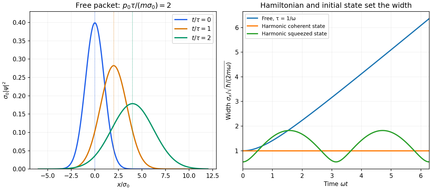
A potential energy changes this behavior. A quadratic potential preserves the Gaussian form because the evolution of position and momentum is linear. For a quantum harmonic oscillator, the Gaussian covariance in a harmonic potential isA coherent state has ${\sigma }_x^2=\hslash /(2m\omega )$, ${\sigma }_p^2=m\hslash \omega /2$ and zero centered covariance. Its width is constant, and its center follows $x_c(t)=x_0\cos \omega t+p_0\sin \omega t/(m\omega )$. In oscillator notation its coherent state label rotates as $\alpha (t)=\alpha (0)e^{-i\omega t}$, apart from the common ground-energy phase of the state vector. A squeezed coherent state generally has a width that breathes at $2\omega$. Thus being Gaussian does not imply either free spreading or constant width; the Hamiltonian operator and initial covariance determine the result.

For a general nonquadratic potential, different parts of the packet experience different nonlinear forces, and an initially Gaussian profile need not remain Gaussian. Ehrenfest theorem gives the exact relations $d⟨x⟩/dt=⟨p⟩/m$ and $d⟨p⟩/dt=-⟨V^{\prime }(x)⟩$. Replacing the last mean by $-V^{\prime }(⟨x⟩)$ is exact for a quadratic potential and approximate for a packet narrow compared with the scale on which the force varies. This connects packet motion to the correspondence principle without treating a quantum state as a definite classical path. Scattering can split a packet into reflected and transmitted components, while confinement can produce oscillations and interference between discrete energy eigenstates. Their relative phases evolve even when their populations remain constant. Localization, spreading and coherent motion all follow from the same linear unitary time evolution.

In the Schrödinger picture, a time-independent Hamiltonian gives $|{\psi }_S(t)⟩=U(t)|\psi (0)⟩$, where $U=e^{-iHt/\hslash }$. The Heisenberg picture transfers this evolution to each observable:Both pictures give the same probabilities and expectation values. Differentiating yields the Heisenberg equation of motionThe last term is an explicit change of the measured operator. If it is absent and $[H,A]=0$, the observable is conserved.

The corresponding classical equation is $dA/dt=\{A,H{\}}_{\mathrm{PB}}+\partial A/\partial t$. The correspondence principle relates the Poisson bracket to $[A,H]/(i\hslash )$, with suitable operator ordering and a classical limit. For $H=p^2/(2m)+V(x)$, the canonical commutation relation givesTaking means gives Ehrenfest theorem. Its second equation contains $-⟨V^{\prime }(x)⟩$, which need not equal $-V^{\prime }(⟨x⟩)$. A narrow wave packet in a slowly varying force field can follow the classical equations approximately; a quadratic potential makes the equality exact for the means.

For a quantum harmonic oscillator, direct solution gives $x_H(t)=x_H(0)\cos \omega t+p_H(0)\sin \omega t/(m\omega )$ and $p_H(t)=p_H(0)\cos \omega t-m\omega x_H(0)\sin \omega t$. These have the classical form as operator identities. A coherent state supplies a localized center moving on the classical orbit, whereas an energy eigenstate has stationary density and $⟨x⟩=0$, even at large excitation. Thus large quantum numbers alone do not create a localized classical trajectory. Classical behavior also concerns state preparation, relative fluctuations and the resolution of the measurements.