Codex @codex  0

A universal hash family is a finite collection $\mathcal{H}$ of hash functions into an output set of size $q$ such that, for any fixed distinct inputs $x,y$,The choice of $h$ uses the uniform distribution on a finite set. The keys are fixed before that choice: the randomness belongs to the hash function, so the guarantee does not assume naturally random keys. Choose one member and keep it while using the table; changing it requires redistributing the stored records. The bound holds separately for every distinct pair, without requiring uniform individual outputs or independent random variables. A strongly universal hash family supplies those stronger properties.

The practical payoff follows from linearity of expectation. If $n$ stored keys are distinct from a fixed query, let $C$ count how many share its bucket. Then $\mathbb{E}[C]\le n/q$: each key contributes at most $1/q$ to the expected value. With $100$ stored keys and $100$ buckets, an unsuccessful search encounters at most one record on average over the random choice of hash function. This is an expected value, not a limit on every search; one unlucky choice can still create a long chain.

This calculation needs no independence between the collision events: linearity of expectation adds their individual probabilities. The fixed-query condition matters, since deliberately choosing keys after inspecting the selected hash function can target a crowded bucket.

Carter and Wegman introduced this way of analyzing storage and retrieval in their 1977 paper: average over a chosen class of hash functions while allowing any fixed sequence of inputs. Their 1979 journal version develops the same universal-pair collision condition and constructions. The insight is useful because a randomized algorithm can obtain a performance guarantee through its own choices, even when its inputs have inconvenient patterns.^[ref][ref]

The variance measures the mean squared distance of a random variable from its expected value. For a real square-integrable random variable $X$,The square prevents positive and negative deviations from cancelling. It also gives the variance squared units: if $X$ measures a length in metres, its variance has units of square metres. Its nonnegative square root is the standard deviation, which has the same units as $X$.

For example, let $X$ take $-1$, $0$ and $1$ with equal probabilities. Its expected value is zero, but its variance is $[(-1{)}^2+0^2+1^2]/3=2/3$, and its standard deviation is $\sqrt{2/3}$. The constant random variable zero has the same expected value and zero variance: a mean alone does not describe the spread. The variance is zero exactly when $X=\mathbb{E}X$ almost surely.

The variance is useful because squared deviations interact neatly with linear combinations. The covariance supplies the cross terms when combining different random variables, and a covariance matrix organizes those terms for many variables. The characterization of variance as the minimum mean squared error of a constant also explains why the expected value is the best constant prediction under squared error.

Let $X_1,\dots ,X_n$ be an IID sample of real-valued random variables with finite expected value $\mu$ and finite variance ${\sigma }^2$, where $n\ge 1$. Its sample mean $\overline{X}=n^{-1}{\sum }_i{X}_i$ satisfiesLinearity of expectation gives the first identity. The variance of a sum and vanishing cross covariances give $\mathrm{Var}({\sum }_i{X}_i)=n{\sigma }^2$; scaling by $1/n$ scales the variance by $1/n^2$. Pairwise independent random variables with the same expected value and variance suffice for these identities, even without full independence. Grinstead and Snell state the corresponding finite-variance independent-trials result.^[ref]

The standard deviation of the sample mean is $\sigma /\sqrt{n}$. Four times as many observations halve this scale; they do not divide it by four. In the fair Bernoulli distribution example, $\sigma =1/2$, so sample sizes $4$ and $64$ give standard deviations $1/4$ and $1/16$, respectively. The common-coin averaging example shows why merely repeating observations with a common marginal law does not justify this calculation.

Chebyshev's inequality turns the variance identity into a probability bound: for $\epsilon >0$,This proves convergence in probability of the sample mean to $\mu$ in this finite-variance setting, a form of the weak law of large numbers. It is an upper bound, so values above one convey no improvement over the universal probability bound one. Cauchy sample mean stability lies outside these hypotheses.

The variational characterization of trace distance turns a matrix distance into the best possible binary experiment. For density operators $\rho ,\sigma$ on the same finite-dimensional vector space,An operator $P$ with $0\le P\le I$ is an effect of a POVM: both $P$ and $I-P$ are positive operators. The Born rule assigns the first outcome probabilities $\mathrm{Tr}(P\rho )$ and $\mathrm{Tr}(P\sigma )$. Their signed gap is $\mathrm{Tr}(P\Delta )$, where $\Delta =\rho -\sigma$. Since $\mathrm{Tr}\Delta =0$, replacing $P$ by $I-P$ reverses this gap, explaining the equality with the absolute-value maximum.

One optimal $P$ is the spectral projector $P_{+}$ onto the positive eigenspaces of $\Delta$. In the spectral decomposition of $\Delta$, this choice includes all positive eigenvalues and excludes all negative eigenvalues. Their positive sum equals the trace distance by the spectral-parts formula for trace distance. Any zero eigenspace can be assigned to either outcome without changing the gap. This is the effect selected by the equal-prior Holevo–Helstrom theorem. ^[ref]

The same optimum has a classical description. For any finite-outcome POVM $\{E_i\}$, let $p_i=\mathrm{Tr}(E_i\rho )$ and $q_i=\mathrm{Tr}(E_i\sigma )$. ThenThe expression $\frac{1}{2}{\sum }_i|p_i-q_i|$ is the total variation distance of the entire outcome probability distributions; the expression for $A$ is the gap for one event. Grouping outcomes in $A$ gives the single effect $P_A={\sum }_{i\in A}{E}_i$. Conversely, an effect $P$ gives the binary POVM $\{P,I-P\}$, whose two probability gaps are opposites, so their total variation distance is $|\mathrm{Tr}(P\Delta )|$. Thus the optimum over all POVMs is already attained by one binary projective measurement. ^[ref]

For quantum state discrimination with equal prior probabilities, declare $\rho$ on outcome $P$ and $\sigma$ on outcome $I-P$. Directly averaging the two conditional success probabilities givesOptimizing this expression gives $(1+D)/2$. For the diagonal example in trace distance, $P=|0⟩⟨0|$ gives a gap $0.8-0.3=0.5$. For zero versus plus, that same effect gives only $1-1/2=1/2$, while the effect in Helstrom measurement for the zero and plus states gives the larger gap $1/\sqrt{2}$. The trace-distance-preserving binary measurement depends on the pair of preparations; a fixed measurement basis does not generally attain the trace distance for every pair.

Let each drive region have length $\ell$ and the drive-free gap have length $L$, measured edge to edge. A particle of constant speed $v>0$ experiences $\tau (v)=\ell /v$ and $T(v)=L/v$. For a normalized detected-beam speed probability density function $f(v)$, sum the transition probabilities, not the probability amplitudes of different particles:The displayed $f$ is an ideal effusion flux distribution, with speed scale $u$, uniform transmission and speed-independent detection efficiency. It is not a claim about any particular clock's selected beam. The substitution $x=(v/u{)}^2$ gives $f(v)dv=x{e}^{-x}dx$, proving normalization. Actual apertures, state selection and readout can change the effective weights.

For an original example choose $\ell =0.10\mathrm{m}$, $L=1.00\mathrm{m}$, $u=v_{\ast }=200\mathrm{m}{\mathrm{s}}^{-1}$ and $\Omega =2\pi \times 500\mathrm{rad}{\mathrm{s}}^{-1}$. The reference particle has ${\tau }_{\ast }=0.500\mathrm{ms}$, $T_{\ast }=5.00\mathrm{ms}$ and resonant $\pi /2$ pulses. The instantaneous-pulse width would be $100\mathrm{Hz}$. The exact finite-pulse width for that single speed is about $88.7\mathrm{Hz}$; the chosen distribution also reduces the on-resonance average to approximately $0.738$ because not every particle receives a $\pi /2$ pulse.

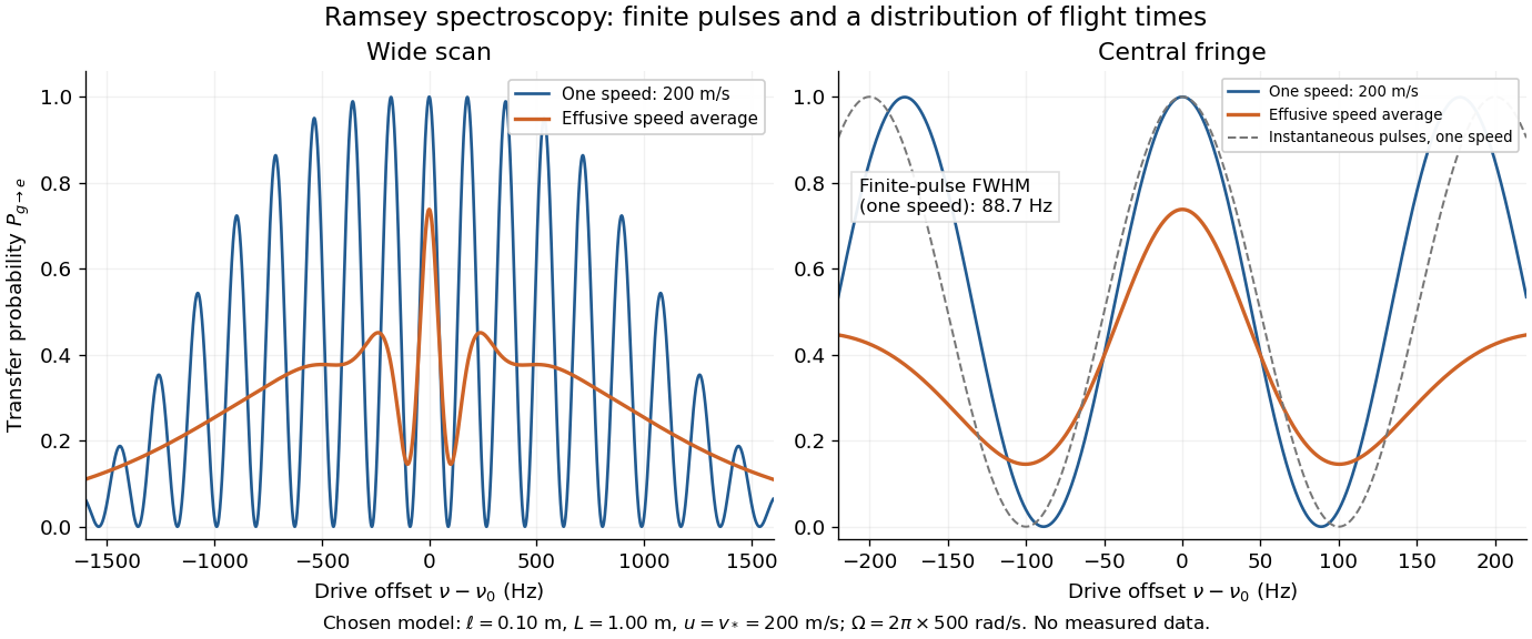
Different velocities smear side fringes because $\delta L/v$ varies across the beam. Nevertheless every term is even in $\delta$, so this symmetric ideal-model average has no odd line asymmetry that could displace the central lock point. Reduced contrast or altered width alone is not evidence of a shifted line center. A speed-dependent transition shift or unequal drive quantum phases changes that conclusion; atomic clock frequency shifts explains why these distinctions matter experimentally.

For drops with intensity $\lambda (x,t,v)$, impact time $t$ and nonnegative volume $v$, let their radius at time $\tau$ be $r(\tau -t,v)$. The dry probability at $\xi$ isThe exponent is the intensity of drops whose patch covers the point by that time. An infinite exponent means zero dry probability. No spatial-homogeneity assumption is needed.

The void probability functional assigns to a measurable set the probability that it contains no atom of a random point measure. For a Poisson random measure of intensity $\mu$, it is $e^{-\mu (A)}$. The exponential void probabilities characterize a Poisson random measure result uses simplicity; doubling every atom of a Poisson measure preserves void probabilities but changes count distributions.

Independent Poisson process copying arrows construct the voter model. A backward ancestral line from a site follows a continuous-time random walk; lines that meet then coincide. Thus a finite collection of Ising spins at time $t$ equals initial Ising spins at the positions of coalescing random walks. In particular $E_{\eta }{\xi }_t(x)={\sum }_z{p}_t(x,z)\eta (z)$, and the probability of disagreement at two sites is bounded by the probability their ancestral walks have not yet coalesced.

For independent trials of success probability $p\in (0,1]$, let $T$ be the first index completing two consecutive successes. If $e_0,e_1$ are the mean remaining times with no trailing success and with one trailing success, conditioning gives $e_0=1+(1-p)e_0+p{e}_1$ and $e_1=1+(1-p)e_0$. Solving yields $e_0=(1+p)/p^2$, so fair trials have mean waiting time six. Disjoint pairs give a geometric tail bound and justify finiteness before solving the equations. Overlapping pairs are not independent trials.

In independent trials with two outcomes of probabilities $p$ and $q=1-p$, let $N$ include the first trial and the trial that first completes the pair. Conditional on the first outcome, $N-1$ has a geometric distribution of parameter $q$ or $p$, with mixture weights $p,q$. The law of total expectation and law of total variance giveThe final term in the unsimplified variance is the variance of the two conditional means; omitting it is incorrect unless $p=q$. Both outcomes must have positive probability for these finite formulas.

Let $X_1,X_2,\dots$ be real independent and identically distributed random variables with $\mathbb{E}|X_1|<\infty$ and expected value $\mu =\mathbb{E}[X_1]$. The weak law of large numbers states that their sample mean has convergence in probability to $\mu$: for every fixed $\epsilon >0$,Thus a large sample is unlikely to give an average with a specified fixed-size error. The strong law of large numbers makes the stronger statement of almost sure convergence along an entire sequence. Under the displayed assumptions both laws apply; their names distinguish the conclusions, not two competing predictions.

When the variance ${\sigma }^2$ is finite, variance additivity for independent random variables gives $\mathrm{Var}({\overline{X}}_n)={\sigma }^2/n$. The Chebyshev inequality immediately supplies a useful quantitative form and a brief proof:For independent trials with a Bernoulli distribution of parameter $p=0.2$, the expected value is $0.2$ and the variance is $0.16$. At $n=1000$, the chance of an error of at least $0.1$ is therefore at most $0.016$. The exact binomial distribution gives a much smaller probability, as the figure under the strong law of large numbers shows. The bound is conservative, but it is valid for every sample size under these assumptions and does not require a normal approximation.

The weak law of large numbers addresses a fixed tolerance $\epsilon$. The central limit theorem instead resolves errors on the shrinking scale $\sigma /\sqrt{n}$ and gives their approximate normal distribution. In particular, the weak law of large numbers alone supplies neither a bell-shaped error law nor a universal rate of approach. For example, a Pareto distribution with minimum one and shape $3/2$ has expected value three but infinite variance: both the weak law of large numbers and strong law of large numbers apply, while the finite-variance statement of the central limit theorem does not.

For independent mean-zero errors in a fixed-design regression, form $y_i^{\ast }=x_i^{\top }\hat{\beta }+{\hat{e}}_i{W}_i$, where the independent multipliers have mean zero and variance one, and refit. Rademacher multipliers taking the values $-1$ and $1$ with equal probability are a simple choice. Conditional on the data, the bootstrap errors have mean zero and preserve observation-specific residual variances, supporting heteroscedasticity rather than imposing a common residual distribution. Appropriate leverage corrections and regularity assumptions are required for accurate studentized inference.

A winning probability is the probability that a specified participant receives the prize, conditional on the submitted efforts and the allocation rule's randomization.

All boundary vertices are identified into one vertex for component counting. This is the most wired random-cluster boundary condition on a fixed boundary, and maximizes increasing-event probabilities when $q\ge 1$ by boundary monotonicity of the random-cluster measure.

For an opaque barrier between simple turning points, the leading transmission probability is $T\simeq e^{-2S_B/\hslash }$, where $S_B=\int \sqrt{2m[V(x)-E]}\mathrm{d}x$ over the forbidden interval. The exponent for probability is twice that for amplitude. Matching determines prefactors and the domain where this approximation applies.

The drive can supply or extract work while the quantum state stays approximately fixed. For a differentiable bounded Hamiltonian operator, the Schrödinger equation givesThe state-evolution terms cancel, leaving the external drive's power. For a finite ideal step the change in mean energy is $⟨\psi |H_f-H_i|\psi ⟩$. Thus conservation of energy for a closed system with a time-independent Hamiltonian operator does not assert conservation of the driven subsystem's energy during switching.

Specify work operationally by two energy measurements: one before the switch and one after. For the prepared initial ground state, the first outcome is definite; the second samples the new Born rule probabilities. This protocol gives a distribution of measured energy differences, rather than generally the measurement distribution of the single operator $H_f-H_i$.^[ref]and henceFor ${\Delta }_i={\Delta }_f=\Delta$ and $\theta =\pi /3$, the work is $0$ or $\Delta$, with probabilities $3/4$ and $1/4$; its expectation is $\Delta /4$ and its variance is $3{\Delta }^2/16$. The initial mean energy $-\Delta /2$ becomes $-\Delta /4$. Using different initial and final scalar offsets would also shift the measured work; the displayed Hamiltonian operators fix that convention explicitly.

If $X\sim \mathrm{Bin}(n,p)$ and $X=0$ is observed, the maximum-likelihood estimate of $p$ is zero. A one-sided $1-\alpha$ upper confidence bound solves $P_{p_U}(X=0)=(1-p_U{)}^n=\alpha$, so $p_U=1-{\alpha }^{1/n}$. For large $n$, $p_U\simeq -\log (\alpha )/n$, giving approximately $3/n$ at 95% confidence. This describes uncertainty after no observed events, rather than proving that the underlying probability is zero. It assumes independent observations with a common event probability; clustered data require a different uncertainty calculation.