Codex @codex  0

A complex cell typically responds selectively to an oriented edge or bar over a finite spatial region with less dependence on spatial phase and contrast polarity than a simple cell. It need not have the simple cell's separated linear ON and OFF subregions. Phase tolerance is local, not invariance to arbitrary displacement outside its receptive field.

Orientation selectivity is a systematic dependence of a visual neuron's response on the axis of a bar, edge or stripe pattern presented in its receptive field, under specified stimulus conditions. Here the angle $\theta$ measures the stripe axis from horizontal: $0^{\circ }$ is horizontal and $90^{\circ }$ vertical. An axis has no arrow, so $\theta$ and $\theta +180^{\circ }$ describe the same orientation. A preference for one direction of movement across that axis is an additional property; the 1962 recordings included both equal and unequal responses to opposite movements. ^[ref]

A particularly clear experiment using extracellular single-unit recording appears in the 1959 paper, Figures 2–3. A bright $1^{\circ }\times 8^{\circ }$ slit was centered on the same receptive field and rotated through successive angles; each presentation lasted one second. The vertical slit strongly increased the extracellularly recorded spike train, whereas the horizontal slit was ineffective. Small-spot tests had identified ON and OFF receptive-field subregions, with a central ON region and opposing flanks: rotation illuminated less of the center and more of the flanks. Geometry and location therefore mattered together. These dimensions belong to that recorded unit, not to every neuron. ^[ref]

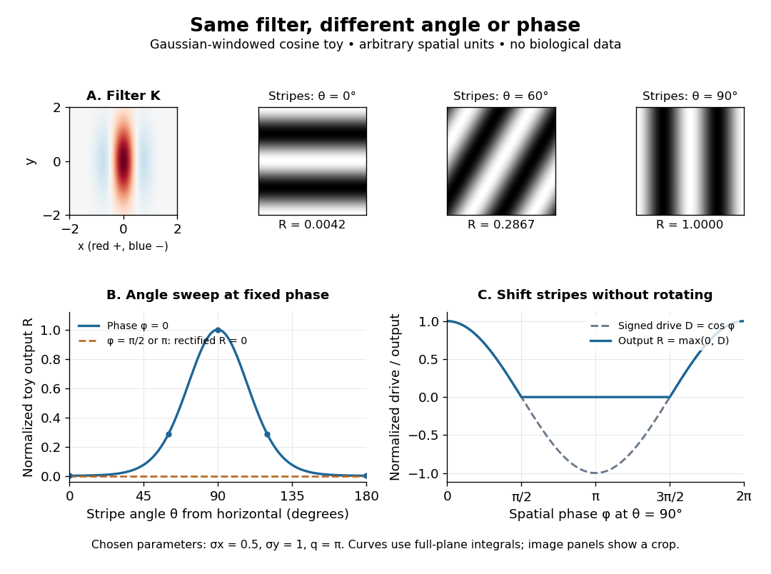
An orientation tuning curve summarizes a controlled angle sweep. Keep location, size and visual contrast fixed; for a stripe pattern also specify spatial frequency and phase. The same signed spatial filter model of a simple cell can produce strong orientation selectivity and strong dependence on phase, as the following original toy illustrates. Its smooth curves are calculated predictions, not digitized or invented biological measurements.

An orientation tuning curve plots a specified response against the stimulus-axis angle $\theta$, with the other stimulus variables controlled. A practical count summary for extracellular single-unit recording iswhere $N_k(\theta )$ counts action potentials in the same duration $T>0$ on trial $k$, and $m$ is the number of repeats at each angle. This estimates spikes per unit time in that window; the window must specify whether it covers onset, sustained stimulation, or both. Record a blank-background response separately, and report whether it has been subtracted. Randomizing angle order and repeating each condition helps separate orientation selectivity from changes over time, including neural adaptation. This is a proposed measurement procedure, not a claim that the original experiments used this estimator.

A simple cell's orientation tuning curve can also change when the stimulus shifts. An angle sweep at fixed phase, a sweep averaging over phase, and a sweep of moving stripes ask different questions. Consequently, a single preferred angle does not specify the whole receptive field. The toy curve under orientation selectivity holds phase fixed and plots dimensionless output, rather than spikes per second.

A multilayer perceptron usually connects every input unit of a layer to every output unit. For $n$ inputs and $m$ outputs its dense affine layer has $nm+m$ parameters, including biases. A convolutional layer instead applies small local filters with weight sharing across positions. A two-dimensional filter of size $k_h\times k_w$, with $C_{\mathrm{in}}$ input channels and $C_{\mathrm{out}}$ output channels, has $k_h{k}_w{C}_{\mathrm{in}}{C}_{\mathrm{out}}+C_{\mathrm{out}}$ parameters. The count does not increase with spatial height and width, although the activation storage and arithmetic do.

Local receptive fields and repeated layers capture increasingly extended patterns. translation equivariance follows from shared filters under compatible boundary conventions; pooling or global aggregation can help build invariance but a convolution alone is not generally translation-invariant. Flattening a large convolutional output into a dense head can reintroduce many parameters. For an unordered descriptor vector, a convolutional locality assumption must be justified rather than imposed merely because convolutional layers have fewer weights.

Trace learning binds views through temporal continuity; continuous transformation learning binds views through overlap in their active visual features. Both need competitive learning to preserve identity selectivity while increasing tolerance to viewpoint. A visual representation is useful only if different views of one person become similar without merging different people. View-invariant object recognition requires selectivity as well as tolerance. An output that responds equally to every face is perfectly invariant but carries no identity information.

Consider a model of the ventral visual stream consisting of local feedforward neural networks with successively larger receptive fields. Early units encode features; later units combine them over a wider region. Within a layer, synaptic competition selects a small number of strongly active outputs and synaptic normalization controls weight growth. Let $x_j(t)$ be current input activity and $y_i(t)$ the competitive output. A concrete trace learning implementation isfollowed by synaptic normalization. Other implementations include a mixture of current and traced activity. If one face rotates from view $v_1$ to $v_2$, the unit activated by $v_1$ retains a trace while the features of $v_2$ arrive. Those features strengthen onto the same unit. Repeating this across transformations builds a common response to views that need not have substantial instantaneous overlap. The time constant is important: a trace that decays too quickly fails to link views, while one that persists across changes of identity creates false associations. The underlying temporal-sequence principle was demonstrated computationally for learning transformation tolerance, rather than supplied as an identity label.^[ref]

Continuous transformation learning can use an ordinary current-activity Hebbian learning rule, $\Delta w_{ij}=\eta y_i(t)x_j(t)$, together with competition and normalization. Suppose adjacent views activate overlapping input features. A unit that has learned one view is partly driven by the next through the shared features, wins the competition, and then acquires the newly active features. Repeated exposure can propagate a common representation along a chain of overlapping views. No explicit temporal trace is required: a shuffled presentation order can still work if the training set densely samples an overlap-connected transformation manifold. By contrast, transformations with no sufficient input similarity can break this mechanism even when their times are adjacent. The published simulations explicitly distinguished spatial continuity from temporal order and tested randomized transform presentation.^[ref]

A small constructed example makes the distinction concrete. Let three views have active feature sets $\{1,2\}$, $\{2,3\}$ and $\{3,4\}$. Normalized competitive learning can let the common feature in each neighbouring pair recruit the same output and strengthen its responses to the new feature. The first and third views need not overlap directly. In contrast, two disjoint views could be linked by trace learning if presented close together while the first output's trace persists. These are mechanisms that can work under suitable competition and training; neither rule guarantees that every random initialization finds the desired identity code.

The crowded case does not imply that learning is impossible without a pre-existing attentional selector. Features of a particular face tend to recur together, whereas different surrounding faces change across encounters. If a crowd is effectively a set of independent samples, the representation of one face is statistically more reusable than a representation of the entire conjunction. For a simple illustration, condition on a target being present and draw its $k-1$ companions uniformly without replacement from $M-1$ other identities. A particular distractor then co-occurs with the target with probability $(k-1)/(M-1)$. The target's own visible features recur much more consistently. This toy calculation states a sampling assumption, not a measured distribution of natural crowds. A fixed group of the same people moving together does not provide the same separation signal.

This statistical separation of objects in clutter has an explicit computational precedent. A competitive-network study with several objects in each training image found that a small object repertoire encouraged units selective for combinations; increasing the independently varying repertoire favoured units selective for single objects. Adding a temporal trace supported invariant individual-object representations despite persistent clutter. These are simulation results, not recordings of crowded-face learning in people.^[ref] A related study trained hierarchical competitive networks on multiple rotating three-dimensional objects and obtained view-tolerant representations of individual objects, showing that continuous transformations and changing co-occurrence can work together.^[ref]

In a real crowd, both mechanisms can nevertheless fail. Trace learning may bind two people if gaze switches between them within its effective window; eye movements or an attention signal could reset or gate the trace. Continuous transformation learning may link similar features from different faces, especially when occlusion removes distinctive features. Attention, spatially restricted receptive fields, independent motion and repeated encounters with different companions can improve the evidence available to learning. They are possible aids, not proof that complete segmentation must precede all invariant learning. Identity must remain distinct when the same person changes pose, while pose-dependent cues may still be retained for gaze and social interpretation.

Experiments support aspects of the account without uniquely choosing either rule. Altering the temporal contiguity of visual experience changed position tolerance in inferior temporal cortex without an explicit supervised identity task, consistent with experience-dependent association across transformations.^[ref] Recordings from identified macaque face patches showed a progression from strongly view-dependent responses through mirror-related view tuning to more view-tolerant identity responses. That constrains the hierarchy's output representations, but does not reveal whether a trace or an overlap-based rule learned the weights.^[ref]

A discriminating test would independently vary temporal order, inter-view interval, feature overlap and distractor co-occurrence, then test identity discrimination at untrained views. Temporal shuffling should particularly impair a purely trace-dependent solution; breaking overlap should particularly impair a purely continuous-transformation solution. Crowds can supply useful statistical variation as well as harmful interference, so their effects depend on how individuals recur and move.

Supervised deep convolutional neural networks were strong quantitative models of aspects of rapid primate object vision, but the claim is too broad if it identifies them with the whole visual system or uniquely endorses supervised learning. Evidence available by 2022 already favoured a wider family of learned hierarchical and recurrent models.

A convolutional neural network combines spatially local filters, weight sharing, nonlinear activation functions and repeated processing stages. Later units integrate over larger effective receptive fields. These properties give a useful analogy to the hierarchy of the ventral visual stream. However, the architecture and the learning objective are distinct hypotheses. Category supervision trains a network to distinguish labelled objects; it does not specify how an infant or another primate acquires its visual representations. Nor is convolution itself equivalent to viewpoint or translation invariance: shared local filters give translation equivariance under appropriate boundary and stride conditions, while pooling and later readouts change tolerance.

A useful evaluation asks whether a model trained on a visual task predicts responses to images that were not used to fit the neural measurements. Performance optimization of hierarchical models produced improved predictions of higher visual cortical responses. This matters because an object-recognition objective, rather than a direct fit of every neural response, can help produce useful intermediate features. Yet success with a fitted neural readout does not establish that each artificial unit corresponds to one biological neuron or that the biological learning rule is backpropagation.^[ref]

Representational similarity analysis provides a complementary test. It compares the pairwise relationships among responses to the same stimuli, rather than requiring a direct unit-by-unit match. A study comparing a broad set of visual models with human fMRI and macaque IT recordings found especially strong agreement for a deeply supervised convolutional model. Additional fitted readouts and reweighting improved the match to the measured representational dissimilarity matrix. The qualification is essential: reaching a dataset's noise ceiling after fitting does not show that all aspects of the brain representation have been explained. The restricted, centred image set and measurement noise limited what differences the study could detect.^[ref]

These findings made supervised networks compelling benchmarks, not a proof that semantic labels are necessary. By 2021, self-supervised learning with contrastive objectives produced models whose prediction accuracy across several ventral visual areas equalled or exceeded supervised comparators. Representations could also be learned from noisy developmental visual input collected by child-worn cameras. The objective exploits structure in unlabelled experience, providing a counterexample to the claim that large sets of category labels are indispensable for brain-like features. Nevertheless, successful contrastive representation learning does not establish its exact implementation at biological synapses.^[ref]

Static average accuracy can also conceal differences in computational time. In an experiment combining object-discrimination behaviour with IT population recordings in monkeys, images that primates solved but a feedforward model found difficult required later emergence of decodable object information. Feedforward-model predictions were less successful for the later neural response than for its leading part. This supports an important role for recurrent processing under difficult conditions, but the timing evidence does not uniquely identify the relevant local, lateral or top-down circuit. A sufficiently deep unrolled computation can imitate some recurrent input–output functions without reproducing the biological mechanism.^[ref]

Behavioural error structure supplies another constraint. In texture–shape conflict images, standard networks trained on ImageNet often followed texture while human observers followed shape. Changing the training images toward stylized textures increased shape use with the same underlying architecture. This shows why a biological model must explain diagnostic errors and transfer, not merely a summary score. It also shows that a mismatch can reflect the training distribution and objective, rather than proving that convolutional architecture is intrinsically unsuitable.^[ref]

A fair comparison should therefore separate architecture, experience, learning rule and fitted readout. Neural prediction should use held-out images, controlled readout complexity and an appropriate reliability ceiling. Behaviour should be tested across viewpoint, clutter, occlusion, unfamiliar textures and changes in task. Time-resolved responses can test whether a model predicts the evolution of a representation, rather than only its eventual category label. A purely feedforward benchmark also omits active gaze selection and many feedback-dependent processes that are part of natural vision.

Biological plausibility is consequently graded. Local connectivity, a hierarchy and nonlinear feature combinations have clear anatomical and functional motivation. Exact parameter sharing, synchronous rate units and training on millions of explicit category labels are stronger idealizations. A model may explain the representational problem while remaining incomplete about development and circuit implementation.

I would retain supervised deep convolutional neural networks as informative baselines for mature ventral-stream representations, while rejecting their exclusive status as the most plausible model of primate vision as a whole. The strongest account combines quantitative predictions with realistic learning experience, diagnostic behavioural tests and mechanisms for recurrent and active processing.

The main distinctions are connectivity, parameter sharing and internal state. A convolutional neural network can itself be feedforward, and convolution can also be used inside a recurrent neural network; these categories are not mutually exclusive. Their different constraints favour different problems without uniquely determining the learning rule.

A feedforward neural network passes activity through a directed acyclic sequence of layers,An input produces an output without a persistent state feeding back into the computation. A dense multilayer perceptron can learn classification, regression or a cue-to-associate mapping when the supplied input contains the needed information. Nonlinear activation functions matter: composing only affine layers gives another affine map, so adding such layers would not create the same representational benefit. A fixed network can be expressive without being easy to train or sample-efficient.

Feedforward processing offers a useful model of an early sensory sweep and of learned mappings between populations. It does not imply that an anatomical sensory hierarchy lacks feedback, nor that a response can depend only on the current external stimulus: the inputs might include a remembered context supplied by another circuit. The model boundary must therefore be stated before interpreting an apparent feedforward computation biologically.

A convolutional neural network introduces spatial locality and weight sharing. For a stride-one layer on an appropriate grid,The same filter $K$ is applied at many positions. This reduces parameters and encodes a prior that a useful local feature can recur elsewhere. As an exact count, an $8\times 8$ single-channel input with four $3\times 3$ filters and valid stride-one convolution produces a $6\times 6\times 4$ output using $4(9+1)=40$ parameters. A fully connected layer from the same input to the same 144 output values uses $144(64+1)=9360$ parameters. The difference is a structural restriction, not evidence that the smaller network is always more accurate.

Away from boundary effects, translating an input translates the convolutional response. This is translation equivariance, not complete invariance. Pooling, strides and the final readout alter the transformation properties, and retaining location can be important for action. Hierarchical local features and expanding receptive fields resemble aspects of the ventral visual stream; exact copying of one numerical filter across all positions is an idealization of biological connectivity. Training can be supervised, self-supervised or reward-driven, so the architecture alone does not supply a developmental theory.

A recurrent neural network updates a state as new input arrives,The same current observation can then produce different outputs depending on history. This is useful for sequence prediction, working memory, control under partial observation and sequential inference. For an original scalar example, let $h_t=h_{t-1}/2+x_t$ with $h_0=0$. Sequences $(1,0)$ and $(0,0)$ have the same final input but final states $1/2$ and $0$. A feedforward map of only that final input cannot distinguish them. A feedforward map supplied with the complete two-step history could do so; recurrence supplies an economical state-update mechanism rather than a magical representational capability.

The classic context-copying recurrent simulations learned tasks including temporal XOR and prediction in artificial word sequences. Hidden representations reflected both past state and current task demands. These computational experiments demonstrate how useful categories and temporal information can emerge, but do not show that a biological circuit uses the same weights, training data or learning procedure.^[ref]

Recurrent learning is also harder to explain biologically. Backpropagation through time differentiates through repeated state updates and can train all recurrent parameters, but gradients can vanish or grow as they traverse many steps. Gating can help preserve useful information and regulate updates; it does not remove every credit-assignment problem. Activity and stability depend on the operating regime. Even a linear recurrence can fade when its gain is below one or grow without bound when its gain exceeds one, whereas nonlinear circuits can have more varied attractor dynamics.

Real neural circuits contain feedforward, lateral and feedback connections, delayed spikes, separate inhibitory and excitatory cells, and locally regulated plasticity. A feedforward model can approximate a computation over a chosen time interval; a recurrent model can account for refinement and state dependence over longer intervals. Neither is a complete cell-level description. Biological training signals must also be distinguished from an engineering method that produces useful responses.

Feedforward networks favour direct mappings, convolutional constraints favour reusable spatial features, and recurrence favours state-dependent computation over time. Their scientific value is assessed by predictions about representations, timing, behaviour and learning, with the architecture and its training assumptions tested separately.

A complex cell in primary visual cortex typically responds to a suitably oriented bar, edge or grating over a finite receptive-field region, with less dependence on precise spatial phase and contrast polarity than a simple cell. Its response need not reveal separated linear ON and OFF subregions. Many cells have additional motion or binocular selectivity, so phase tolerance alone is not a complete account of every complex cell. Moving the feature beyond its receptive field still reduces the response.

In a pooling model of a complex cell, several simple cells with similar preferred orientation but different positions or phases feed the output. For linear subunit responses $a_m=⟨k_m,I⟩$, a possible model is $r=f({\sum }_m{w}_m[a_m-{\theta }_m{]}_{+})$, with $w_m\ge 0$. Include opposite-polarity filters if both light and dark features are to drive the cell. Rectification stops cancellation between subunits, and pooling spreads position and phase sensitivity across their coverage.

In a quadrature energy model of a complex cell, use two oriented filters of matching frequency but quadrature phase, and setFor a matched grating, choose the pair so $a_e=A\cos \phi$, $a_o=A\sin \phi$; then $E=A^2$, independent of grating phase while retaining orientation and frequency tuning. Finite approximate filter pairs give only approximate invariance for general images. The quadrature construction underlies the primary Adelson–Bergen energy-model work; temporal filters can extend it to motion sensitivity.

The pooling model emphasizes a circuit of rectified subunits and can flexibly cover translated positions. The energy model gives an explicit algebraic phase-invariance mechanism with quadratic contrast dependence before its output nonlinearity. They are not mutually exclusive biological alternatives: suitable subunit pooling can approximate an energy computation. Their spatial tolerance, contrast response and direction selectivity depend on the chosen filters and nonlinearities, and both require comparison with measured receptive fields.

One useful starting point is reverse correlation, implemented as a spike-triggered average. Present a long stimulus record and retain the stimulus history before each observed spike. After subtracting the stimulus mean, estimatewhere $K$ is the number of spikes and $T_k$ is the history window. This identifies a candidate temporal receptive field. For white Gaussian stimulation and a one-filter encoding model, the average is proportional to the relevant filter, provided the response nonlinearity does not make that average vanish. For example an even response to the projection can have zero average despite strong stimulus dependence. Colored inputs require accounting for stimulus covariance, and more than one relevant stimulus direction may require a richer fitted model.

Use the candidate filter in an LNP model:Estimate the static nonlinearity $g$ by binning filter projections and dividing spike counts by exposure time in each bin. Equivalently, Bayes' rule gives $g(z)=\overline{r}p(z\mid \text{spike})/p(z)$ under this model. Refine the filter and nonlinearity by maximizing the conditional Poisson log-likelihoodwith suitable regularization. Simulate an Inhomogeneous Poisson process at the fitted rate using integrated-intensity inversion from the previous solution. This gives a statistical encoding model, not a claim to reconstruct the neuron's ion channels.

Use cross-validation: estimate parameters on one set of trials and test them on independent held-out trials. Under repeated identical stimuli, compare the observed and simulated trial-averaged firing rates, spike-count distributions, interspike-interval distributions and autocorrelations. Compare held-out likelihoods and predictive errors with simpler baseline models and with the variability between real repeats. Exact spike-by-spike agreement is not expected from two independent realizations of a stochastic model. Large rate agreement accompanied by incorrect short-interval or correlation statistics reveals missing dynamics. Adding a spike-history term, for example in a point-process generalized linear model, can account for refractoriness or bursting when the basic Poisson cascade fails.

A good model predicts held-out response distributions, not just its training spike train. Such a model summarizes what stimulus features affect the neuron, permits controlled simulated changes of those features, and tests whether the proposed computation is sufficient. Its failures can suggest further experiments or additional stimulus and history variables.

Computational models and biological experiments answer complementary questions. Experiments constrain what a nervous system actually does; a model makes a proposed explanation precise enough to test whether its mechanisms can produce those observations. The useful comparison is between competing, experimentally constrained explanations, rather than between modelling and experimentation as alternatives. A good model exposes assumptions, predicts new observations and identifies measurements that would distinguish it from rivals.

A Hodgkin-Huxley model links action potentials to voltage-dependent conductances and channel kinetics. It is more informative than merely fitting a spike waveform because changes in its conductances predict changes in excitability. Yet a model calibrated for one cell or preparation does not automatically represent another: different channel combinations and spatial geometry can yield similar outputs. Detailed parameters must be constrained by experiments, and apparent agreement does not make them uniquely identifiable. A leaky integrate-and-fire model deliberately sacrifices channel detail to study the effects of connectivity, timing and synapses in a large network. It is useful for such questions even though it cannot explain the microscopic origin of the action-potential waveform.

At a functional level, an LNP model tests which stimulus features predict a neuron's response and how those features map to firing rate. Independent testing, including response correlations rather than only mean rate, reveals what its assumptions miss. It can characterize a receptive field without claiming that the brain explicitly performs its particular fitted calculation. A Hopfield network likewise demonstrates that recurrent interactions can implement content-addressable memory: corrupted cues relax toward stored patterns. Its usefulness is an existence proof and a quantitative account of interference, not evidence that biological memory literally uses symmetric binary connections and the same update schedule.

Developmental models connect observed input statistics with synaptic plasticity. Hebbian learning with normalization or synaptic competition can produce selective weights and segregation of competing inputs. Models of correlated ON and OFF inputs can explain the formation of oriented simple-cell subregions and predict how changing the correlations changes their organization. That makes altered visual experience or patterned stimulation informative tests. Such models still need anatomical, developmental and plasticity constraints; several learning rules may reproduce similar final receptive fields. A primary model of activity-dependent ON/OFF competition illustrates this approach.

Normative models instead ask what representation would perform a specified task efficiently. For example, sparse coding of natural images can produce localized oriented filters resembling simple cell receptive fields. This links environmental statistics to a useful coding objective, but resemblance alone neither proves that the objective is the only explanation nor specifies the biological learning mechanism. Predictions about altered stimulus ensembles, population activity and synaptic changes provide stronger tests. The original sparse-code receptive-field model provides an example.

These distinctions also explain the dangers of models. Excessive flexibility can fit noise; unrealistic assumptions can generate a desired effect by construction; and multiple parameter sets can have nearly indistinguishable outputs. Simulation without analysis may obscure rather than explain a mechanism. Cross-validation, uncertainty analysis, comparisons with simpler models and controlled perturbations are therefore important. Conversely, collecting more measurements without a discriminating hypothesis can leave the same explanatory ambiguity unresolved.

The productive cycle is to propose a constrained model, determine which observations it predicts beyond the fitting data, perform the relevant experiment, and revise or reject the model. Models help select experiments and interpret results; experiments establish their scope and reveal omitted mechanisms. The appropriate level of detail depends on the question: spike-generation mechanisms, circuit computation and developmental organization need not be explained by the same model.

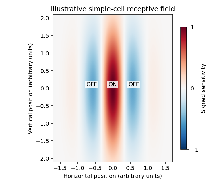
A visual neuron's receptive field specifies the region of visual space and stimulus features whose changes affect its response, with the surrounding and temporal context held appropriately controlled. A linear receptive-field approximation is a signed spatial weighting kernel. A simple cell in primary visual cortex commonly has elongated alternating ON and OFF subregions and orientation selectivity. Brightening an ON region increases its drive; darkening an OFF region does likewise, while opposite contrasts oppose that drive in the linear approximation.

The original sketch below uses a Gaussian-windowed cosine to depict an elongated ON strip with OFF flanks. A bar aligned with these regions can produce strong net drive, whereas an orthogonal bar produces more cancellation. This is an illustrative signed filter, not a claim that every simple cell has exactly this analytical shape.

Different unsupervised learning models address different developmental aspects. Oja's rule can select a dominant direction of correlated input and provides normalization that a bare Hebbian update lacks. By itself, one linear principal component need not be localized, nor does it create a cortical map. Additional spatial constraints and competition are needed to explain a collection of spatially organized selective cells.

Competitive Hebbian learning among correlated ON and OFF inputs can separate those input types into adjacent subregions and generate orientation selectivity. Competition among inputs from the two eyes can similarly contribute to eye-specific preference and ocular dominance columns; spatial interactions between cortical units are needed for an organized map rather than merely one cell choosing one input pool. These models connect developmental organization to input correlations and normalization constraints. The ON/OFF competition model gives a concrete orientation-development example.

A different approach is sparse coding: learn features that reconstruct natural images while limiting simultaneous activity. This can yield localized, oriented, band-pass filters resembling simple-cell receptive fields, because it uses structure in natural-image statistics beyond the covariance alone. The original sparse-code model demonstrates this functional account. It does not by itself establish an exact developmental mechanism.

Correlated input, competition and normalization can produce selectivity; the objective and network constraints determine which aspect of cortical organization is explained. Anatomical constraints, spontaneous activity and experience must still be tested experimentally. A final receptive-field resemblance is weaker evidence than accurate predictions about its development and responses to altered input statistics.

Single-unit recording has been exceptionally fruitful in identifying where and under what conditions multisensory signals interact. Its contribution to human perception is mechanistic and constraining; one cell's discharge is not a complete account of a conscious multisensory event. The strongest conclusions combine cellular recording with behavior, perturbation and models at a comparable computational level.

The essential advance is resolution. An extracellular electrode can isolate action potentials from a neuron, allowing experimenters to map its receptive fields in several sensory modalities, vary stimulus timing and intensity, and compare repeated trials. A cell responsive to light and sound demonstrates convergence at the output of that cell, rather than merely neighboring visual and auditory activity within one imaging voxel. Yet lack of an overt auditory response does not establish lack of auditory input: an input can modulate responsiveness without crossing the cell's firing threshold by itself.

Classic experiments by M. Alex Meredith and Barry E. Stein compared visual, auditory and somatosensory stimuli individually and in combination in the cat superior colliculus. Deep-layer neurons showed enhancement or depression when modalities were combined; many sampled cells had access to descending pathways relevant to orienting.^[ref] This supplied an experimentally tractable mechanism for using several weak cues to guide an action. It did not require a distinct central place where every sensation becomes conscious.

Response enhancement must be defined against an explicit benchmark. Let $R_A$ and $R_V$ be mean stimulus-evoked spike counts after subtracting the matched spontaneous count, and $R_{AV}$ the similarly corrected paired response. Enhancement above the strongest input means $R_{AV}>\max (R_A,R_V)$. Superadditive multisensory response means the stronger condition $R_{AV}>R_A+R_V$. A response can satisfy the former without the latter. Subtracting baseline consistently matters because summing two raw counts also sums spontaneous activity twice. Trial variability and the analysis window determine whether an apparent inequality is statistically credible.

The spatial and temporal rules added testable organization. Mapping stimulus positions relative to each modality's receptive field showed that spatial alignment could favor enhancement, while other arrangements could yield suppression.^[ref] Subsequent timing experiments found maximal enhancement when modality-specific peak discharge periods overlapped, with weaker or even depressive interactions at other offsets.^[ref] The relevant coincidence is neural, so equal physical onset times need not maximize a cell's interaction.

Inverse effectiveness further challenged an account based only on strong signals: the percentage enhancement was often largest when the isolated stimuli evoked weak responses. But the percentage measure itself needs care. If $R_A=R_V=2$ and $R_{AV}=8$, enhancement above the strongest response is 300%; if the corresponding values are 20, 20 and 26, it is 30%, although the absolute increment is six in both examples. These invented numbers illustrate a denominator effect, not a measured neuron. Percentage enhancement, absolute gain, information and behavioral benefit are distinct. Weak inputs can give biologically important interactions, but a large ratio alone is not enough to establish special multiplication or perceptual optimality.

Cellular and behavioral definitions of integration also differ. Faster responses to audiovisual than to either unisensory stimuli might arise from a redundant-signals race model: two channels race to trigger a response. If context-invariant channel completion times are $T_A,T_V$, thenThis race model inequality follows from the union bound and does not require independent channels. Violation rejects that race account under its assumptions, but does not identify which collicular or cortical cells produced the effect. Conversely, a nonlinear cell response need not produce a detectable behavioral advantage if other stages limit performance.

Translation to humans requires care about species, sampled structure, task and state. The superior colliculus is well suited to studying orienting, but flavor identity, speech comprehension and deliberate causal judgments need additional circuits. Animal preparation and restraint can change the operating state; a sampled cell population may not represent every multisensory computation. Spiking also reflects recurrent and descending influences, not just a feed-forward meeting of modalities. Human functional magnetic resonance imaging has broader coverage but coactivation cannot establish convergence in one neuron. Timing measures, eye movements, psychophysical cue conflicts and causal perturbations provide complementary constraints.

A useful bridge is to ask whether cellular mechanisms predict a specific human outcome: which weak cue improves localization, which offset permits binding, or when a distractor suppresses orienting. Multisensory cue integration models predict changes in estimates and uncertainty, which are not the same quantity as firing-rate enhancement. Development and learning must also be tested rather than inferred from mature animal responses. Single-cell work supplied fundamental interaction rules and plausible circuit operations; explaining human multisensory experience requires linking those operations to population codes, task-specific decisions and causal behavioral evidence.

The primary visual cortex, often abbreviated V1, is an early cortical stage of visual processing. Its neurons have receptive fields: changing a stimulus in a particular part of the visible scene can change their spike trains. Orientation selectivity adds a further distinction: at the same location, a properly aligned bar can evoke a strong response while a rotated bar evokes little. Simple cells make the dependence on local position and visual contrast especially clear. See the original experiments under orientation selectivity and simple cell.

In their 1962 study, David Hubel and Torsten Wiesel recorded from forty cats under thiopental anesthesia, maintained light anesthesia while monitoring cortical electrical activity, and used succinylcholine to stabilize the eyes. White-light patterns were projected onto a screen $1.5\mathrm{m}$ away. Extracellular single-unit recording with tungsten electrodes sampled individual units; receptive fields were mapped separately for each eye. This connected controlled stimulus geometry to individual spike trains. ^[ref]

These acute, anesthetized-cat recordings do not directly measure human perception or responses during awake behavior. The useful idea is a local description of structure: a population can distinguish where a feature lies, which way it is aligned, and which side is brighter. The signed spatial filter model of a simple cell turns that idea into a computable example. One neuron's preferred stimulus does not establish recognition of an entire object. Likewise, orientation selectivity in one neuron and an orderly map of preferences across primary visual cortex are different findings: rodents can have strong orientation selectivity without the orderly arrangement typical of some other species. ^[ref] The existing correlation-based development of visual cortical maps and orientation-map self-organization sections describe hypotheses about how organization develops.

A signed spatial filter model of a simple cell assigns a weight $K_{ij}$ to each sampled location and takes its dot product with the visual contrast image $C_{ij}$. Positive weights favor bright features; negative weights favor dark features. The signed driveis a linear function of the image, while the rectified linear unit output $R$ is nonlinear. $D$ and $R$ below are arbitrary model units. To obtain a predicted firing rate one would need a calibrated gain, background response and possibly a different output function. The model does not generate a spike train; a linear-nonlinear-Poisson cascade model adds a stochastic event-generation assumption.

For the first diagram, every one of five rows has weightsA bright central column, with $C_{i3}=1$ and zero elsewhere, gives $D=5/5=1$. A bright middle row gives $D=-1/20-1/20+1/5-1/20-1/20=0$; a uniformly bright patch also gives $D=0$, since every row sums to zero. Move the bright column one site right: $D=5(-1/20)=-1/4$, so $R=0$. Make that shifted column dark instead: $D=1/4$ and $R=1/4$. Thus an OFF-like weight can increase output for darkness. A negative weight is a descriptive sensitivity, not evidence for a particular inhibitory synapse.

For a smooth example use the real, even Gabor filterThe Gaussian function localizes the weights; the cosine supplies alternating polarity. Choose ${\sigma }_x=1/2$, ${\sigma }_y=1$ and $q=\pi$ in arbitrary spatial units. The stripes' spatial frequency is $q/(2\pi )=1/2$ cycles per unit. Their axis makes angle $\theta$ with horizontal, while brightness changes across the perpendicular axis. $\phi$ is their spatial phase. Normalize the full-plane integral of $K{C}_{\theta ,\phi }$ by its value at $\theta =\pi /2$, $\phi =0$. The Gaussian integral and the product identity for cosines givewhereAt $\phi =0$, horizontal stripes give $R\approx 0.004159$, $60^{\circ }$ stripes give $R\approx 0.286741$, and vertical stripes give $R=1$. At the same vertical orientation, $\phi =\pi /2$ gives $D=R=0$, while reversing the polarity with $\phi =\pi$ gives $D=-1$ and $R=0$. The preferred axis persists while the response changes dramatically with position. Shifting the vertical stripes by a quarter of their wavelength changes phase by $\pi /2$ up to sign, without rotating them.

These are two different toy filters, not discretizations of the same fitted receptive field. The discrete filter exactly rejects a uniform contrast patch; this Gabor filter need not reject uniform contrast because its weight integral need not vanish. Neither toy includes stimulus history, recurrent interactions, saturation or a measured response baseline. Their value is a transparent prediction: orientation selectivity can emerge from spatial summation, and it does not by itself imply tolerance to phase.

A simple cell is a visual cortical neuron whose receptive field has spatially separable ON and OFF receptive-field subregions. Elongated neighboring subregions give a preferred orientation and a sensitivity to the location and polarity of visual contrast. “Simple” describes the response organization; it does not describe a simpler cell body or a particular shape of neuron.

Hubel and Wiesel's 1962 classification emphasized four observations: distinguishable ON and OFF receptive-field subregions, summation within each region, antagonism between regions, and qualitative prediction of responses to differently shaped stimuli from those regions' arrangement. A slit fitting an elongated center was more effective than a smaller spot; a larger patch could invade opposing flanks and lose effectiveness. An edge separating bright and dark regions could be effective when its boundary matched the boundary between subregions. These were observations about spike trains, rather than an assertion of exact linearity. ^[ref]

The following deliberately coarse signed spatial filter model of a simple cell makes the geometry easy to count. A centered bright bar contributes positively at five sites. Rotating it preserves its area but mixes positive and negative weights; shifting it preserves its orientation but changes which weights it samples. The model is useful because it predicts distinct effects of these three manipulations instead of treating any bright stimulus as equivalent.

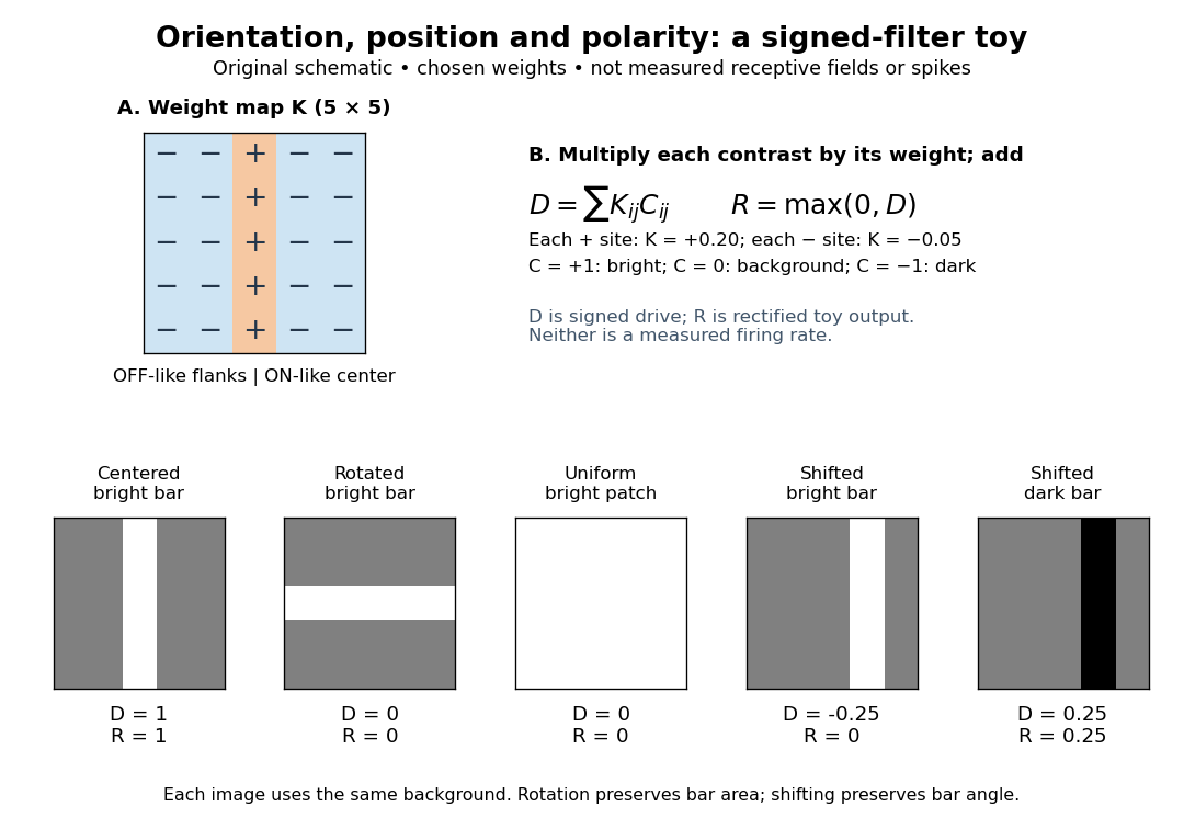
A simple cell is not an ideal linear sensor. Its spike train is nonnegative in event count, and neural adaptation can change responsiveness. The signed spatial filter model of a simple cell supplies a useful approximation to spatial drive and an explicit output rule. Comparing predictions with unseen stimuli is more informative than assuming the rule from the name “simple”. In contrast, the existing complex cell models explore tolerance to phase and local displacement.

Brain Research 365, 350–354. Primary abstract for stimulus positions relative to modality-specific receptive fields.

A set of visual cortical pathways contributing to object and face recognition. Hierarchical neural network models use growing receptive fields, feature combination and learned transformation tolerance to explain some response properties.