Consider the original analytic initial value problemHere and are dimensionless variables in a stipulated mathematical model. The trajectories below are exact solutions of a differential equation, with no measured data or empirical parameter fit. For , the Bernoulli power substitution givesThe integrating factor is . Direct differentiation gives , independently checking the transformation. The linear exists for every real , while the nonlinear solution of a differential equation uses only the interval containing where :For , , so its absolute value decreases toward zero. The lost zero solution of a differential equation is recovered by substitution into the original equation. Since is locally Lipschitz in everywhere, the Picard-Lindelöf theorem ensures uniqueness through every finite point, including . Thus a nonzero trajectory never meets or crosses zero at a finite .
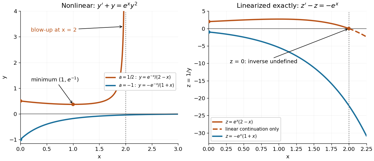
Two Bernoulli trajectories and their exact linearized coordinates
. The initial conditions are in orange and in blue. Left: the positive trajectory reaches finite-time blowup at , while the negative trajectory approaches zero. The vertical axis clips the positive curve at ; this is a display limit. Right: the corresponding trajectories satisfy . The dashed orange continuation past solves the first-order linear differential equation but cannot extend the original positive initial value problem across blowup. Details.
For , the exact solution of a differential equation is on . It first decreases, reaches a local minimum , then increases without bound. At the endpoint,The finite-time blowup comes from a simple zero of at , where , rather than from a singular coefficient in the first-order linear differential equation. The same algebraic expression for is negative on , but that is a separate solution of a differential equation on a disjoint interval; infinity supplies no finite joining value. For , on , giving a distinct decaying branch whose finite blowup is instead in the past.
The direction field also explains the positive turning point. Its nullclines are and , becauseAbove the positive nullcline, ; between it and zero, ; below zero, . The moving nullcline is not a solution of a differential equation: its derivative is , whereas the prescribed slope there is zero. The trajectory crosses it at , exactly its local minimum.
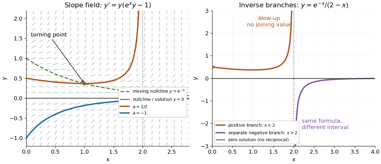
The Bernoulli direction field and the disconnected inverse branches at blowup
. Left: the direction field, its two nullclines, and the exact and trajectories. Right: has a positive branch on and a negative branch on ; the excluded point separates them. The zero solution of a differential equation belongs to the original equation but has no finite reciprocal coordinate. The branches continue beyond the plotted vertical limits. Details.
Articles by others on the same topic
There are currently no matching articles.