A Bernoulli differential equation is a first-order ordinary differential equation of the displayed form, with and continuous functions on an interval and a fixed real exponent . A nonlinear power can hide a first-order linear differential equation: on a suitable branch, the Bernoulli power substitution removes it exactly. The transformed solution of a differential equation can be completely regular even when recovering produces finite-time blowup.
For example, the reciprocal Bernoulli equation with finite-time blowup becomes under . The initial conditions and select a positive trajectory blowing up at and a negative trajectory tending to zero as , respectively. The integrating factor exposes both behaviors with the same short calculation.
The cases and are already first-order linear differential equations: respectively , with the zeroth-power term interpreted as the constant , and . There is no need for a nonlinear change of variable; for , would discard the unknown entirely. For other exponents, the substitution must respect the domain of exponentiation and may lose the zero solution of a differential equation.[ref]
1.5 Substitution. Notes on Diffy Qs, §1.5.2 Bernoulli equations: substitution v equals y to the power 1 minus n; n equals 0 or 1 is already linear; Example 1.5.1 selects the positive root using its initial condition
Let q be continuous and strictly positive, with a constant a. A nonnegative solution of a differential equation may stay zero until any prescribed point and become positive afterwards. For , defineand set before . The Bernoulli power substitution verifies the equation after . Continuity of q gives , so the joining derivative is zero and the equation also holds at the join. These different waiting times give nonunique solutions from zero. The right side lacks Lipschitz continuity as a function of y near zero, so the uniqueness conclusion of the Picard-Lindelöf theorem does not apply there.
For on a positive real branch, put and . The Bernoulli power substitution gives . Its integrating factor is , yieldingThe resonant case needs an extra factor x because the forcing has the same exponential dependence as the homogeneous solution. Recover only on an appropriate real branch. The case is already a first-order linear differential equation; a zero solution or zero-crossing behavior must be checked in the original equation separately.
For arbitrary real , work first on an interval where . Define exponentiation by , using the real logarithm. The change of variable is differentiable and invertible there, and the chain rule givesMultiplying the Bernoulli differential equation by yields the first-order linear differential equationThis is an exact transformation of nonzero solutions of a differential equation on the chosen branch; it is valid far from any reference state and does not discard higher powers as a local linearization would.
Given the initial condition , the integrating factor and transformed solution of a differential equation areThe product rule verifies . Recover only on the connected component of containing , inside the original coefficient interval. The first-order linear differential equation can have a longer existence interval than this inverse transformation allows.[ref]
1.4 Linear equations and the integrating factor. Notes on Diffy Qs, §1.4 Linear equations and the integrating factor: product derivative, formula (1.4), and Remark 1.4.1 on existence throughout a coefficient-continuity interval
Negative values need a separately justified real branch. For integer , the required powers are real and differentiable for too, but the inverse must retain the sign selected by the initial condition. For , represents either or ; both square roots are taken of positive . For , retains the sign directly. For a general noninteger exponent, use the positive branch unless a specific differentiable real negative branch has been established. Never evaluate a real fractional power of a negative value merely because the linear formula has become negative.
Division by excludes . When and the original real power is defined at zero, is an additional solution of a differential equation and must be checked in the original equation. When , the equation as written is undefined at zero. On a positive branch the right-hand side is locally Lipschitz in , so the Picard-Lindelöf theorem gives local uniqueness. At zero, the same hypothesis needs a fresh check: it holds for the polynomial example, whereas for a nonzero power coefficient prevents local Lipschitz continuity there. If , the inverse sends for , but sends for . The latter endpoint can lead to finite-time extinction in a sublinear Bernoulli equation, where the original equation determines how to join to zero.
Consider the original analytic initial value problemHere and are dimensionless variables in a stipulated mathematical model. The trajectories below are exact solutions of a differential equation, with no measured data or empirical parameter fit. For , the Bernoulli power substitution givesThe integrating factor is . Direct differentiation gives , independently checking the transformation. The linear exists for every real , while the nonlinear solution of a differential equation uses only the interval containing where :For , , so its absolute value decreases toward zero. The lost zero solution of a differential equation is recovered by substitution into the original equation. Since is locally Lipschitz in everywhere, the Picard-Lindelöf theorem ensures uniqueness through every finite point, including . Thus a nonzero trajectory never meets or crosses zero at a finite .
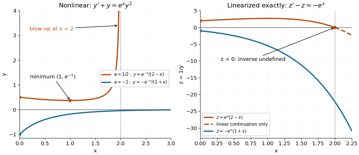
Two Bernoulli trajectories and their exact linearized coordinates
. The initial conditions are in orange and in blue. Left: the positive trajectory reaches finite-time blowup at , while the negative trajectory approaches zero. The vertical axis clips the positive curve at ; this is a display limit. Right: the corresponding trajectories satisfy . The dashed orange continuation past solves the first-order linear differential equation but cannot extend the original positive initial value problem across blowup. Details.
For , the exact solution of a differential equation is on . It first decreases, reaches a local minimum , then increases without bound. At the endpoint,The finite-time blowup comes from a simple zero of at , where , rather than from a singular coefficient in the first-order linear differential equation. The same algebraic expression for is negative on , but that is a separate solution of a differential equation on a disjoint interval; infinity supplies no finite joining value. For , on , giving a distinct decaying branch whose finite blowup is instead in the past.
The direction field also explains the positive turning point. Its nullclines are and , becauseAbove the positive nullcline, ; between it and zero, ; below zero, . The moving nullcline is not a solution of a differential equation: its derivative is , whereas the prescribed slope there is zero. The trajectory crosses it at , exactly its local minimum.
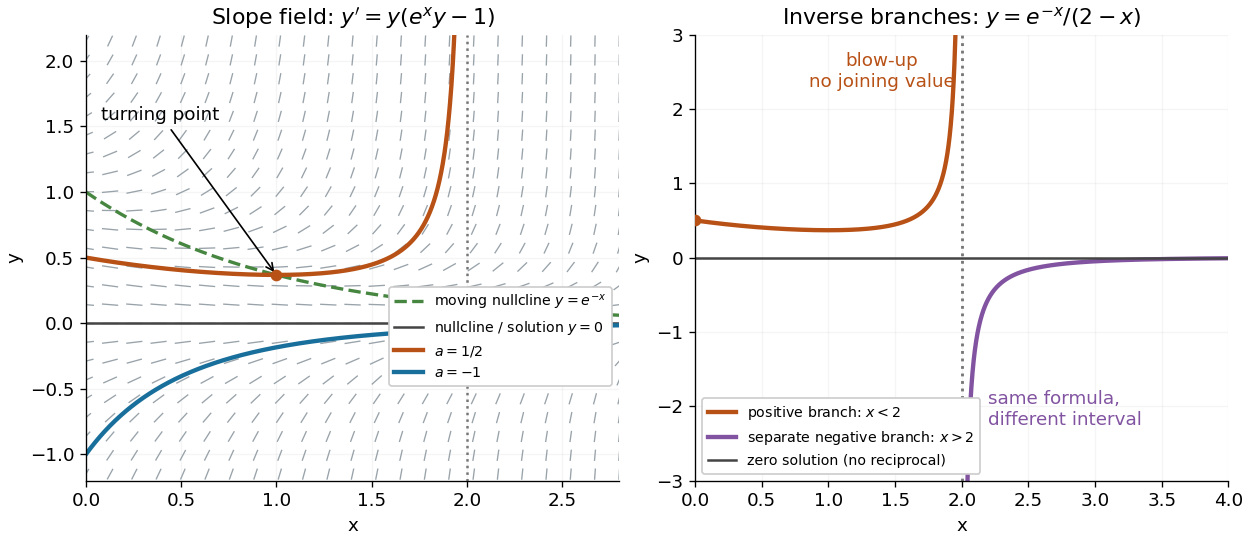
The Bernoulli direction field and the disconnected inverse branches at blowup
. Left: the direction field, its two nullclines, and the exact and trajectories. Right: has a positive branch on and a negative branch on ; the excluded point separates them. The zero solution of a differential equation belongs to the original equation but has no finite reciprocal coordinate. The branches continue beyond the plotted vertical limits. Details.
For , and , put while . Then . If , decreases to zero at the displayed finite time. The positive branch joins the zero solution with zero first derivative, giving a nonnegative forward solution. The equilibrium at zero is one-sided stable even though the vector field is not locally Lipschitz continuous there; the positive equilibrium is unstable.
Articles by others on the same topic
There are currently no matching articles.