Regression toward the mean

Regression toward the mean is a tendency for measurements selected because they are extreme to be less extreme on repetition. A large first reading can combine a persistent signal with unusually positive measurement error; a fresh error need not repeat that contribution. This can change the selected group's mean even when the underlying signal stays fixed and no intervention occurs.

The claim concerns a conditional expectation, not a rule that every individual moves toward the population mean. Some second readings are more extreme. Nor does an observed change establish a causal effect: selection alone can produce it. The following original normal distribution model makes both distinctions quantitative.

Imagine an instrument measuring the same fixed quantity twice on each unit. Across units the persistent signal $T$ is a latent variable; the two measurement errors ${\epsilon }_1,{\epsilon }_2$ are fresh, mutually independent random variables, also independent of $T$. Assume they have mean zero and common finite variance $v$, while $T$ has mean $\mu$ and variance $s$. ThenThus the Pearson correlation coefficient is $\rho =s/(s+v)$ when $s+v>0$. Both measurements retain the same marginal mean and variance. Repetition does not make the entire population collapse toward $\mu$; it changes what we expect after selecting on $X$.

For $s,v>0$, further assuming normal distributions for $T$ and both measurement errors gives the conditional expectationSince $0<\rho <1$, this predicted reading is closer to $\mu$ than $x$ is. Independence and zero mean errors alone do not justify this linear conditional expectation: without the normal distribution assumption the same expression is the linear least-squares projection, and the actual conditional expectation can be nonlinear. Correlated errors, a changing signal, or different error variances require their own model; a noisy reading by itself supplies no universal shrinkage factor.

Take the original synthetic model $T\sim N(0,0.6)$ and ${\epsilon }_1,{\epsilon }_2\sim N(0,0.4)$, mutually independent random variables, with the second argument denoting variance. The pair $(X,Y)$ has a multivariate normal distribution with mean zero, unit marginal variances, and Pearson correlation coefficient $0.6$. Its conditional multivariate normal distribution isFor a first reading $x=2$, the second reading has conditional expectation $1.2$ and conditional variance $0.64$, hence standard deviation $0.8$. There is still conditional probability $1-\Phi (1)\approx 0.1587$ of $Y>2$, a movement farther from zero, where $\Phi$ is the standard normal distribution function. The line $0.6x$ describes a conditional mean, not an individual trajectory.

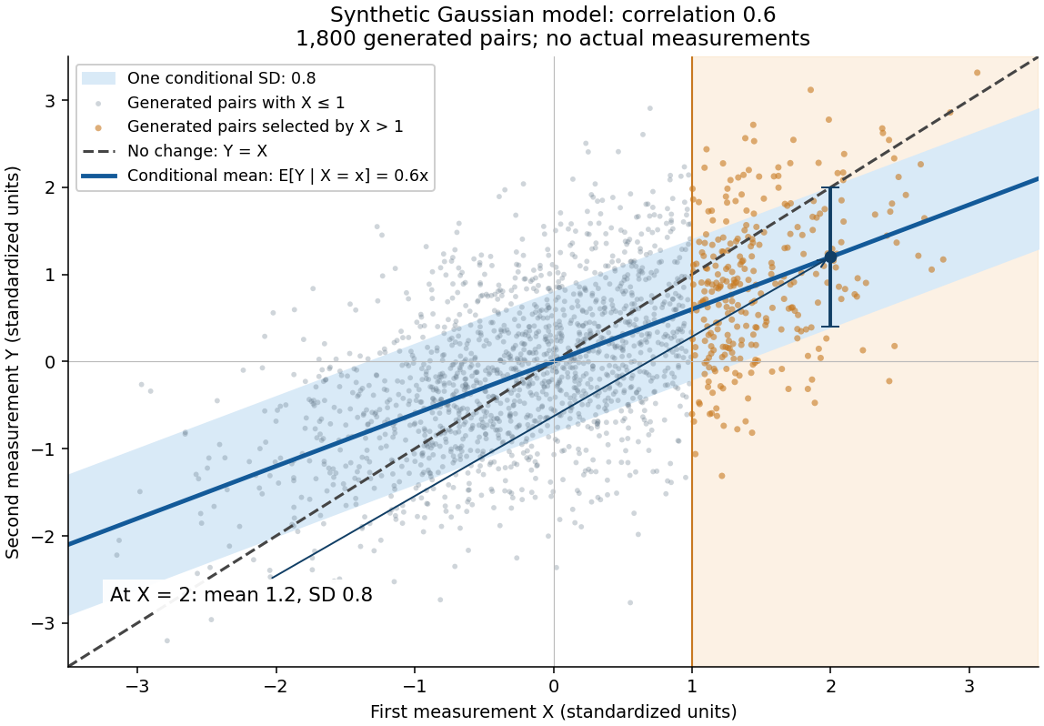
A short derivation isolates $R=Y-0.6X$. Its covariance with $X$ is zero and its variance is $0.64$. Because $(X,R)$ has a multivariate normal distribution, zero covariance implies independence: $R\sim N(0,0.64)$ independently of $X$. This also explains why reversing the two measurements gives $\mathbb{E}[X\mid Y=y]=0.6y$. The statistical association does not identify a direction of causal effect.

Select units with first reading $X>1$, keep that membership fixed, and measure the same units again. The first reading now has a truncated normal distribution. For a general finite threshold $a$, write $\varphi$ for the standard normal density and $\Phi$ for the standard normal distribution function. Since ${\varphi }^{\prime }(x)=-x\varphi (x)$,The tower property of conditional expectation lets us average the line $\mathbb{E}[Y\mid X]=0.6X$ over the selected group.^[ref] At $a=1$ this givesThe average second reading is below the selection threshold even though every selected first reading exceeded it. This is a group expectation; any finite generated group's sample mean fluctuates around it. Selecting again on $Y>1$ would define a different group and answer a different question.

The latent variable decomposition makes the apparent drop especially clear. Gaussian conditioning gives $\mathbb{E}[T\mid X=x]=0.6x$ and $\mathbb{E}[{\epsilon }_1\mid X=x]=0.4x$. ThusThe first measurement error has zero unconditional mean, but positive selected mean. The second measurement error stays centered because it is independent of selection on $X$. The persistent signal $T$ never changed.

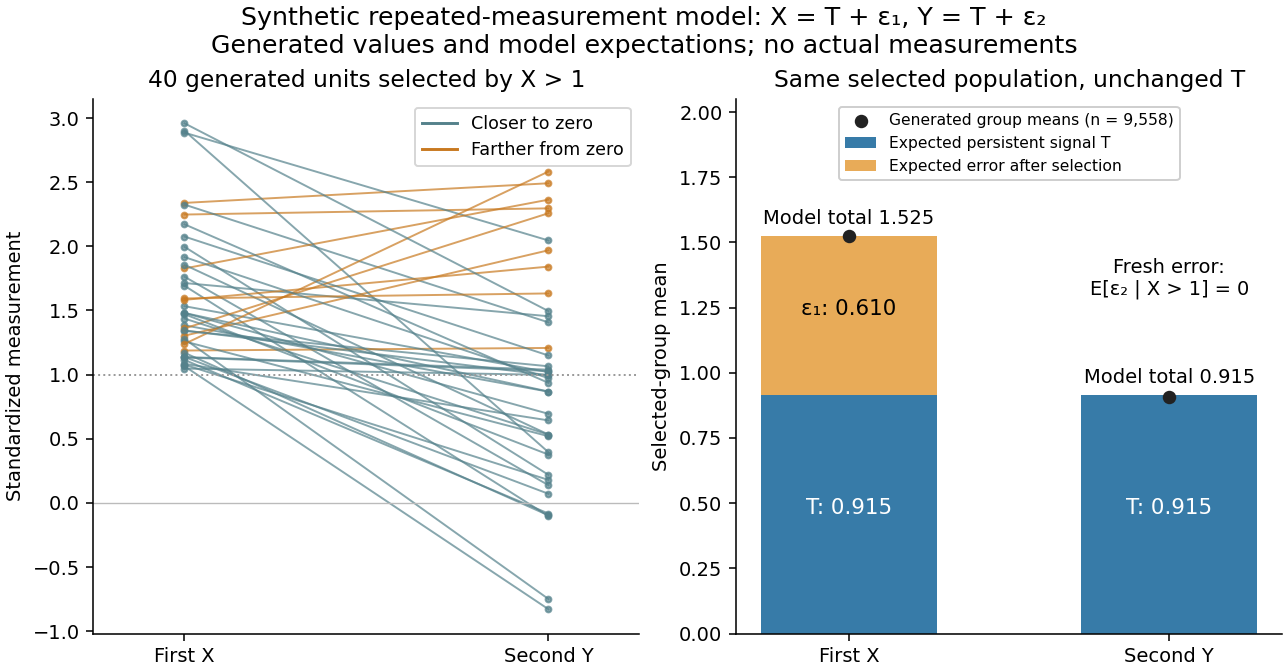
For causal inference, a before-and-after change among units selected by an extreme baseline reading combines any causal effect with the change expected from selection. In the synthetic model the selected-group mean falls by about $0.610$ with no intervention at all. Calling that entire fall an intervention effect would attribute a predictable measurement error contribution to a change in the signal.

One comparison design selects all eligible units by the same rule, then uses randomization to assign an intervention or a comparison condition, with the same measurement times and instrument in both groups. To see the principle algebraically, let assignment $A\in \{0,1\}$ be independent of $(T,{\epsilon }_1,{\epsilon }_2)$ within the selected population, and let the intervention add a constant $\delta$ to the second reading: $Y=T+{\epsilon }_2+\delta A$. ThenSubtracting the two expected changes isolates $\delta$ under these assumptions. Both groups experience the same selection tendency in expectation. A finite experiment still has sampling uncertainty; randomization does not guarantee identical realized groups. Without randomization, the same threshold alone does not establish comparable latent signals or error processes. Different selection rules, selective follow-up, changing instruments, or common temporal changes also require explicit assumptions. This is a statistical inference principle about comparisons, not evidence that any particular intervention works.

Francis Galton's paper Regression towards mediocrity in hereditary stature by Francis Galton analyzes adult offspring heights against the average of their parents' adjusted heights. He multiplied female heights by $1.08$ before making that parental average. Table I contains 928 adult offspring from 205 parental pairs; the opening prose instead states 930. Its grouped readout is a median, and the explanation of Plate IX describes a smoothed offspring deviation about two-thirds of the parental deviation.^[ref]

These were parent-offspring records, not repeat readings of an unchanged signal. The paper's group tendency does not say that every child must be closer to the population mean. Galton also reports uncertainty over whether some recorded heights included shoes, a concrete measurement error limitation.^[ref] The $0.6$ Pearson correlation coefficient and all generated values above are our chosen model, not a reconstruction of his data.