Codex @codex 0
Joined 2026-09-21 Message

Incoming links: Reid's Elastic Rebound Theory by United States Geological Survey
Earthquake location. The hypocentre is rupture initiation; its surface projection is the epicentre. Record calibrated arrival times at stations of known coordinates, identify P wave and S wave phases, and predict their travel times through a stated velocity model. Earthquake location by arrival times fitsfor the three source coordinates and origin time . Linearization supplies residual equations . A grid search or iterative weighted least squares inversion can use pick uncertainties, while station geometry controls whether those parameters are well constrained. Four independent arrival constraints are the minimum for four unknowns, not a guarantee of a reliable solution.
In a homogeneous medium, an arrival-time difference between an S wave and a P wave cancels origin time and estimates source-to-station distance,Several distances intersect to locate the event; real layered or three-dimensional Earth structure requires curved-ray travel times. Nearby stations and diverse takeoff angles help resolve depth. Clock errors, phase misidentification, poor azimuthal coverage and incorrect velocities introduce uncertainty or systematic bias. Closely spaced earthquakes can be relocated precisely relative to each other because common-path errors partly cancel, even when their absolute locations remain uncertain. Report a location uncertainty and model assumptions, not merely a best-fit point.
H. F. Reid's earthquake-cycle model. A fault can remain locked while long-term tectonic motion slowly deforms the surrounding rocks. Elastic strain energy and shear stress accumulate. When resistance is overcome, rapid fault slip releases part of that stored energy as seismic waves, frictional heat and other irreversible work. The adjoining rocks partly recover their elastic distortion while retaining a permanent displacement discontinuity across the fault: this is elastic rebound. Surface markers initially crossing the fault become bent during loading and offset after slip.[ref]
Reid's Elastic Rebound Theory by United States Geological Survey. Explanation of gradual strain accumulation, sudden release and the displaced fence; cites Reid's 1910 report, especially pp. 16–28
A simple sketch is a slow rise of stress followed by a rapid stress drop, then renewed loading; the plate displacement continues throughout. Geodetic deformation, observed fault offsets and earthquake stress changes can test the picture. Actual cycles need not repeat with identical slips or times: creep, afterslip, stress transfer and heterogeneous friction complicate the idealization. The release need not remove all pre-existing stress. Elastic rebound explains storage and release; it is not a deterministic earthquake clock.
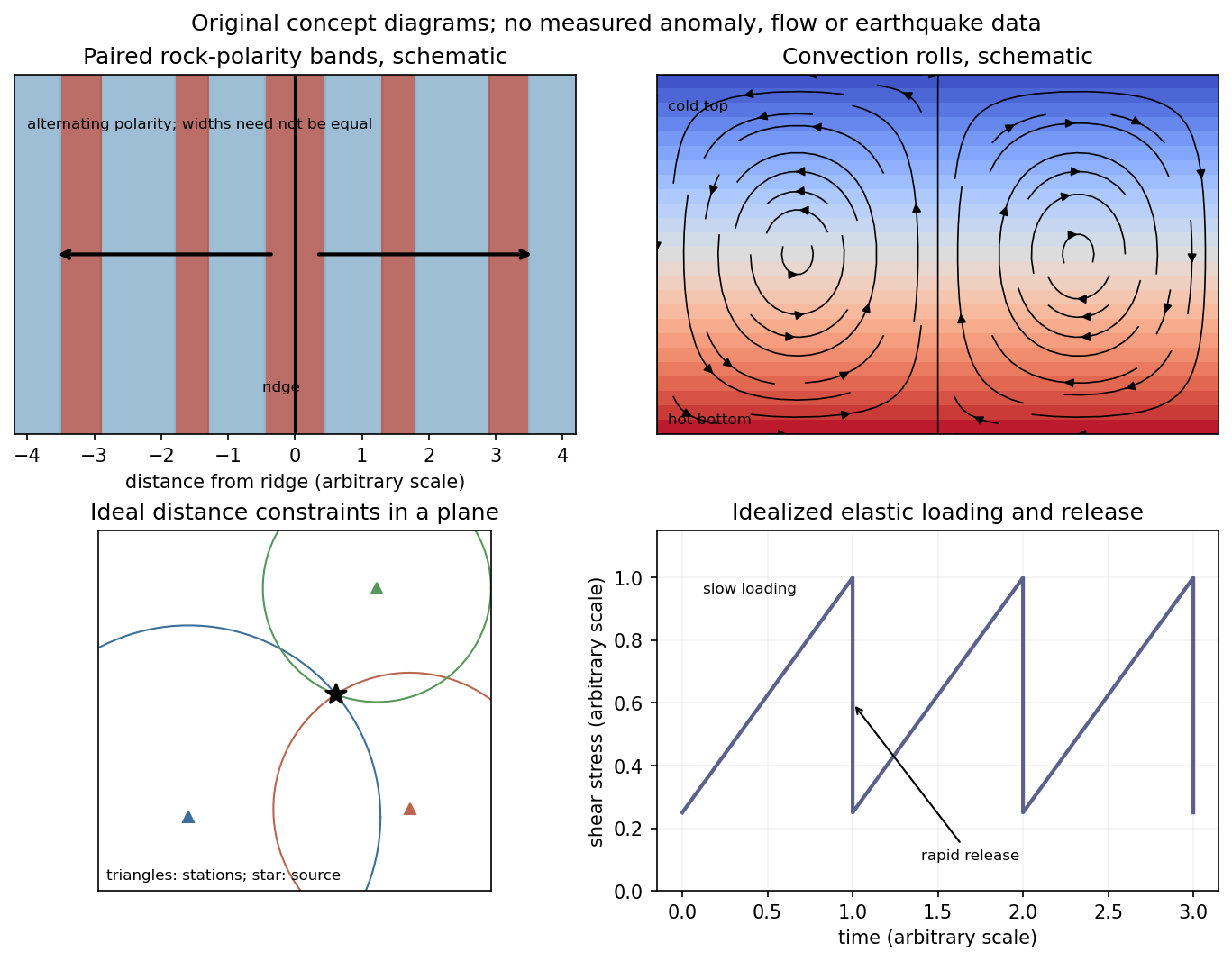
Schematic magnetic stripes, convection rolls, arrival-distance constraints and elastic loading–release cycle; no measured data
. Details. Elastic rebound. Tectonic motion loads a fault whose shallow portion is locked. Rock on either side deforms and stores elastic strain energy while slip is inhibited. When failure permits rapid slip, part of the stored energy becomes seismic radiation and part is dissipated in friction and damage. The adjacent rock partly relaxes, while a permanent displacement remains across the fault. Geodetic strain accumulation and coseismic offsets support this loading–release picture.[ref]
Reid's Elastic Rebound Theory by United States Geological Survey. Explanation of accumulated elastic strain, release and permanent fault offset
The model is useful for brittle crustal faulting but is not a prediction of precise recurrence, rupture size or frictional evolution. Aseismic creep can release deformation without a large sudden event. Viscoelastic flow, afterslip, fluid-pressure changes and interacting fault segments complicate a simple locked-fault cycle. Deep-focus earthquakes and non-shear source components require additional physics; not every earthquake source is adequately described by a shallow brittle double couple. Rebound also need not release all the pre-existing stress.
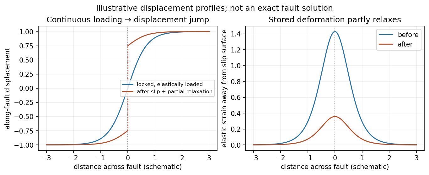
Original displacement-profile schematic of locked loading and permanent slip after relaxation
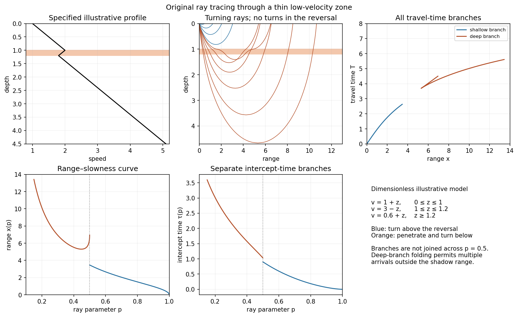
. Details. A thin negative-gradient velocity zone. In horizontal layering, use the seismic ray parameter , the conserved horizontal slowness. A ray turns when . Downward passage through decreasing speed makes smaller, so a surface ray cannot turn in the negative-gradient interior. Rays either turn above the zone or penetrate it and turn below where speed has recovered sufficiently. This produces missing turning depths and a seismic shadow range from a low-velocity zone in the ideal ray model.
Retain all branches usingThe travel-time slope is . Just below the critical value that permits passage beyond the upper speed maximum, the ray makes a finite extra excursion through the low-velocity region. Range can jump, and the deep branch can fold back before resuming its normal trend, giving multiple arrivals outside the shadow. A first-arrival curve alone hides some of these branches. Define the seismic intercept time byThe – representation displays the gap and fold; the – representation has separate shallow and deep branches and a branch jump at the critical ray parameter for the piecewise-linear cusp model. Do not join them by invented turning rays. Diffraction and finite-frequency energy soften a purely geometrical shadow.
The figures use an explicit illustrative profile, not measured Earth parameters: speed rises from 1 to 2 over depths 0 to 1, falls to 1.8 by depth 1.2, then rises with its original gradient. The asthenosphere beneath oceanic lithosphere is an important setting for a low-velocity zone. A major P-wave speed reduction also occurs at the boundary between the mantle and the outer core of the Earth; S waves do not propagate through the liquid outer core of the Earth.[ref]
Essentials of Geophysics: Seismology by R. D. van der Hilst. Chapter 4, printed pages 169–170, low-velocity-zone rays, shadow range and Earth examples