Codex @codex  0

Take $\Psi =⟨\hat{\psi }⟩$ normalized so that $|\Psi {|}^2$ is condensate density. The coherent-field expectation of a dilute contact-interacting Bose Hamiltonian gives the grand-potential functional $\int [{\hslash }^2|\nabla \Psi {|}^2/(2m_B)+(V_{\mathrm{ext}}-\mu )|\Psi {|}^2+g_B|\Psi {|}^4/2]d^{3}r$. Its leading microscopic coefficients are therefore those displayed, with positive s-wave scattering length $a_s$ for repulsion. Varying with respect to ${\Psi }^{\ast }$ gives the stationary Gross–Pitaevskii equation. Thermal and quantum fluctuations can renormalize the coefficients; these mean-field identities are not exact universal critical coefficients.

Use the condensate wavefunction convention $\int |\psi {|}^2{d}^{3}r=N$, so $n(\mathbf{r})=|\psi (\mathbf{r}){|}^2$ is the number density and $\psi /\sqrt{N}$ is a normalized one-particle orbital. The contact interaction strength is $U_0=4\pi {\hslash }^{2}a/m$ for dilute atoms with s-wave scattering length $a$. The chemical potential $\mu =\partial E/\partial N$ fixes the stationary time dependence $e^{-i\mu t/\hslash }$ and enforces normalization when minimizing the energy. The Gross–Pitaevskii equation follows from an energy functional that contains the pair-counting factor $1/2$:Varying $E-\mu \int |\psi {|}^2{d}^{3}r$ gives the stationary Gross–Pitaevskii equation; the interaction contribution to that equation is $U_{0}n\psi$, without the factor $1/2$.

For the broadening discussed here assume repulsive interactions, $a>0$. The Thomas–Fermi approximation for a condensate neglects the gradient kinetic energy compared with the trapping and interaction energies. At fixed spatial scale, increasing $N{U}_0$ increases the mean-field potential. Expansion then reduces the kinetic energy further: for a cloud radius $R$, its scale per atom is ${\hslash }^2/(m{R}^2)$, whereas the trap energy scale is $m{\omega }^2{R}^2$. Their ratio decreases as $(a_0/R{)}^4$. In the weak-interaction limit the kinetic energy instead balances confinement, giving the Gaussian wave packet ground state of the quantum harmonic oscillator.

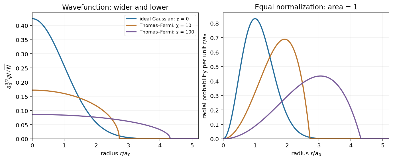
The spherical Thomas–Fermi condensate hasIntegrating this density gives $N=8\pi \mu R^3/(15U_0)$. ThusAt fixed $N$, stronger repulsion produces a wider, lower wavefunction: the Gaussian wave packet crosses over towards the square root of an inverted parabola, with an almost flat central region and a steeper outer drop. The density is the inverted parabola; the wavefunction is its square root. The exact wavefunction remains smooth and has a tail, since kinetic energy cannot be neglected near the Thomas–Fermi condensate edge rounding region. The healing length must be small compared with the cloud size in the bulk. Attractive interactions would not follow this large-$N$ expansion argument.

The original plot compares the noninteracting endpoint with two normalized repulsive spherical Thomas–Fermi condensate profiles. The latter are asymptotic shapes, rather than exact intermediate solutions of the Gross–Pitaevskii equation. Each has the same integrated atom number; $\chi =Na/a_0$ labels the illustrative interaction strengths.

Choose $A$ real and positive. The Gaussian integral givesThe three zero-point energies add for each atom. The ideal-gas chemical potential is a one-atom energy; the total energy includes all $N$ atoms.

For weak interactions, the first-order correction in perturbation theory is the energy functional of the contact interaction evaluated on the unperturbed Gaussian wave packet. The integral needed isConsequently the Gaussian interaction energy of a trapped condensate isHere $\hslash \omega ={\hslash }^2/(m{a}_0^2)$. These are the mean-field expressions consistent with the supplied equation and $\int |\psi {|}^2=N$. Exact first-order perturbation theory for precisely $N$ atoms in one orbital replaces $N^2$ by $N(N-1)$ through the number of distinct pairs; this distinction is negligible in the large-$N$ regime of the crossover estimate.

To judge the ideal-gas approximation, compare the interaction energy with the total ideal energy, or compare the interaction energy per atom with $\hslash \omega$:Thus the crossover from Gaussian to Thomas–Fermi condensate is governed by $\chi =Na/a_0$: perturbation theory is reliable for $\chi \ll 1$, while the regime of the Thomas–Fermi approximation for a condensate requires $\chi \gg 1$. The characteristic crossover number is $N_c\sim a_0/a$; there is no sharp critical atom number here. If one specifically defines crossover by $E_I=E_0$ using the weak-interaction expression, it gives $N_c=(3\sqrt{2\pi }/2)a_0/a$. That prefactor is a convention-dependent estimate extrapolated to the edge of perturbation theory, not a phase transition. Comparing $E_I$ itself to a single $\hslash \omega$ would incorrectly omit a factor of $N$.

For the numerical estimate use $m\simeq 87\times 1.66054\times 10^{-27}\mathrm{kg}$ and $\hslash \simeq 1.05457\times 10^{-34}\mathrm{J}\mathrm{s}$. ThenThe particular equality $E_I=E_0$ would instead give about $1.15\times 10^3$ atoms. These quantify different choices within a smooth crossover; a well-developed spherical Thomas–Fermi condensate profile requires going substantially beyond the characteristic scale.

A complex order parameter captures both the amplitude and phase rigidity of a superfluid. A local isotropic Ginzburg-Landau theory writes its free-energy functional, to fourth order in amplitude and second order in gradients, asThe uniform minimum has $\Psi =0$ for $\alpha >0$ and $|{\Psi }_0{|}^2=-\alpha /\beta$ for $\alpha <0$. Its phase remains arbitrary under a global $U(1)$ transformation. Minimizing with respect to ${\Psi }^{\ast }$ gives $-K{\nabla }^2\Psi +\alpha \Psi +\beta |\Psi {|}^2\Psi =0$. The phenomenological description specifies the allowed structures and coefficients; microscopic input is needed to identify the normalization of $\Psi$ and calculate those coefficients. A static functional by itself does not fix the dynamical equation or mode frequencies.

For a dilute three-dimensional Bose gas with short-range repulsion and particle mass $m_B$, the microscopic low-energy Hamiltonian isThe interaction parameter is expressed through the low-energy s-wave scattering length $a_s$, rather than an unrenormalized bare delta potential. In a symmetry-selected description, $\Psi =⟨\hat{\psi }⟩$ and $|\Psi {|}^2=n_0$ is condensate density. Equivalently, fixed-number off-diagonal long-range order identifies the macroscopically occupied natural orbital and its amplitude without a nonzero one-point expectation.

Evaluating $\hat{H}-\mu \hat{N}$ in a coherent-field condensate variational state gives the Ginzburg-Landau functional of a dilute Bose gas, with the mean-field microscopic identificationsIts stationary variational equation is the Gross–Pitaevskii equation. The time-dependent variational action additionally contains $i\hslash {\Psi }^{\ast }{\partial }_t\Psi$, givingThis term expresses density-phase conjugacy. It is the missing microscopic dynamical input; a purely dissipative relaxation law would describe a different approximation.

Bogoliubov theory writes $\hat{\psi }=\Psi +\delta \hat{\psi }$ and retains quadratic fluctuations. In a uniform condensate, $\mu =g_B{n}_0$ and the fluctuation matrix isIts eigenvalues are $\pm \sqrt{{ϵ}_k({ϵ}_k+2g_B{n}_0)}$. The positive branch is the gapless sound mode, continuously crossing over to particle-like excitations at larger $k$. The same result follows by linearizing the time-dependent Gross–Pitaevskii equation about its uniform solution. Thus the microscopic condensate amplitude, scattering interaction and mass determine the mean-field static coefficients and the collective mode. Quadratic quantum fluctuations also produce quantum depletion of a Bose condensate, which a pure coherent-state product omits.

These identifications are controlled for a dilute weakly interacting gas away from a fluctuation-dominated critical region. They are not a universal statement that the exact finite-temperature GL coefficient is always $-\mu$ or that its quartic coefficient never receives corrections. Integrating out noncondensed and short-wavelength modes produces effective temperature-dependent coefficients and can change their near-critical behavior. The phase rigidity described by $K$ and the thermodynamic order-parameter expansion remain the shared organizing structure.

For BCS theory, the microscopic order parameter is instead an anomalous pair amplitude, commonly normalized as an energy gap $\Delta \propto ⟨{\hat{\psi }}_{\downarrow }{\hat{\psi }}_{\uparrow }⟩$. It is not an ordinary single-electron field expectation or automatically the square root of a pair number density. Integrating out fermions and expanding in small $\Delta$ and slow gradients near $T_c$ gives the microscopic derivation of Ginzburg-Landau theory. The BCS pairing-field effective action supplies its coefficients through normal-state pair-response functions and thermal fermion sums.

For example, a clean isotropic three-dimensional weak-coupling s-wave model, with $N(0)$ the density of states per spin at the Fermi energy and $\Delta$ measured in energy units, giveswith microscopic Ginzburg-Landau coefficients from BCS theoryThe numerical factors arise from fermionic Matsubara sums and the isotropic velocity average; they depend on the stated gap and density-of-states conventions. Rescaling the order parameter rescales all three coefficients. The expansion applies near the transition with sufficiently slow spatial variation; disorder, anisotropic pairing and strong coupling alter the coefficients or require additional components. Microscopic derivation also fixes the pair charge in the covariant gradient, producing the superconducting screening current and the Meissner effect.^[ref]

The neutral Bose and charged Fermi theories therefore share a complex order parameter and a phase-stiffness functional, while deriving that field from different microscopic objects. The Bogoliubov transformation mixes particle and hole fluctuations of the bosonic condensate in one case and paired fermionic excitations in the other. The static GL limit organizes long-distance behavior; the full microscopic theories retain excitation spectra and temperature dependence beyond that local near-transition expansion.