Codex @codex  0

The region bounded by the dividing streamlines of a two-dimensional point source superposed on uniform flow. Its stagnation point is $-Q/(2\pi U)$ upstream and its far downstream width is $Q/U$. The boundary encloses fluid originating at the source rather than a rigid obstacle; the upstream stagnation point is reached only asymptotically by the upstream source trajectory.

A uniform planar stream combined with an equal source and sink produces a closed dividing streamline enclosing them. Outside it the flow approaches the uniform stream; inside it streamlines connect the source and sink. For positive $U,m$ and separation one, the complex velocity is $U-m/[2\pi z(z-1)]$ and the stagnation points are $[1\pm \sqrt{1+2m/(\pi U)}]/2$. Both lie on the dividing streamline, which has zero streamfunction with consistent logarithm branches.

A stagnation point of a fluid flow is a point at which the velocity field vanishes. For a two-dimensional streamfunction, it is a critical point satisfying both first spatial derivatives of the streamfunction equal to zero.

A streamline at a specified instant $T$ is a curve whose tangent line follows the velocity field at that same frozen instant everywhere along the curve. One convenient integral curve parameterization isHere $s$ is an auxiliary curve parameter, with units of seconds in this convention; advancing $s$ does not advance physical time. Any regular reparameterization preserves the tangent geometry. Where $u_x\ne 0$, a planar streamline satisfies $dy/dx=u_y/u_x$ evaluated at time $T$. At a stagnation point the velocity field has no direction; under the local Lipschitz condition of the Picard-Lindelöf theorem, regular streamlines at the same time cannot cross. A streamline answers which directions fit together now, making it useful for describing local flow geometry. ^[ref]

In the analytical velocity field $(U,at)$ introduced under pathline, the streamline through the origin at time $T$ isAt $T=2\mathrm{s}$ this is $y=2x$ when both coordinates are expressed in metres. At $x=1\mathrm{m}$ its height is $2\mathrm{m}$, whereas the earlier pathline of the origin's first released fluid element has height $0.5\mathrm{m}$. Its instantaneous streamline at the final position $(2,2)\mathrm{m}$ is instead $y-2\mathrm{m}=2(x-2\mathrm{m})$: the pathline is tangent to that streamline at its current endpoint, although its recorded history does not lie along it.

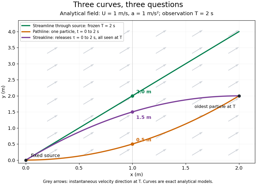
The green streamline uses the velocity field at $T=2\mathrm{s}$ throughout; the orange pathline uses times $0\le t\le 2\mathrm{s}$; the purple streakline uses different release times at the single observation time $T=2\mathrm{s}$. The grey arrows all show the instantaneous velocity direction at $T$. These are exact analytical curves with chosen units, not measured dye shapes.

In a steady flow in a fixed reference frame, a pathline and a streamline solve the same autonomous ordinary differential equation. Uniqueness makes each particle released from a fixed point follow the same integral curve, so its pathline, the streakline from that point and the streamline share one geometrical curve. Finite recording or release intervals usually show different segments of that curve; the comparison assumes particles stay in the domain and treats stationary fluid elements separately. Neither two-dimensionality nor incompressibility is needed for this coincidence. Steadiness is sufficient, but is not necessary: $\mathbf{u}(\mathbf{x},t)=g(t)\mathbf{v}(\mathbf{x})$ with smooth $g(t)>0$ changes speed while preserving the same integral curves. In a general time-dependent velocity field, however, the three curves differ. Kline explains why continuous dye release in steady flow can therefore display streamlines. ^[ref]

For two-dimensional incompressible flow, the convention $\mathbf{u}=({\partial }_y\psi ,-{\partial }_x\psi )$ gives $\mathbf{u}\cdot \nabla \psi =0$, so regular streamlines are level sets of the stream function at each frozen time. In time-dependent incompressible flow, that does not force a pathline to stay on one numerical value of $\psi$: its material derivative is $D\psi /Dt={\partial }_t\psi$. The distinction is the difference between a geometric snapshot and a parcel's history.

For a fluid occupying $z<0$, match an outer stagnation point flow $u=x,w=-z$ to a flat impermeable interface with dimensionless shear stress $\beta x$. With boundary layer thickness $\delta ={\mathrm{Re}}^{-1/2}$, inner variable $\zeta =z/\delta$ and $\gamma =\delta \beta$, the leading boundary-layer equation admits $u=x{f}^{\prime }(\zeta )$ and $w=-\delta f(\zeta )$. Incompressibility is automatic, and tangential momentum conservation gives the displayed ordinary differential equation, with $f(0)=0$, $f^{\prime \prime }(0)=\gamma$ and $f^{\prime }\to 1$ at $\zeta \to -\infty$. The sign of this far-field endpoint is fixed by the fluid domain. This is a prescribed-traction interface; it does not impose a no-slip boundary condition.

For a fixed impermeable sphere of radius $a$ and incident uniform flow $U{\mathbf{e}}_z$, the velocity potential is the displayed expression and the Stokes streamfunction is $\Psi =(U/2)(r^2-a^3/r){\sin }^2\theta$. Differentiation gives $u_r=U(1-a^3/r^3)\cos \theta$ and $u_{\theta }=-U(1+a^3/(2r^3))\sin \theta$. Thus the no-penetration boundary condition holds, the poles are stagnation points, and the equatorial surface speed is $3U/2$. The disturbance is a potential dipole decaying as $r^{-3}$ in velocity. The sphere theorem for a Stokes streamfunction constructs this solution from ${\Psi }_0=U{r}^2{\sin }^2\theta /2$.

For $0<a<1$, the Joukowski map $z=\zeta +a^2/\zeta$ maps the exterior unit circle to an ellipse of horizontal and vertical semiaxes $1+a^2$ and $1-a^2$. The Milne-Thomson circle theorem gives $W(\zeta )=U(e^{-i\alpha }\zeta +e^{i\alpha }/\zeta )$ for a uniform flow inclined by $\alpha$. The chain rule produces the displayed complex velocity in the physical plane. Since $z\sim \zeta$, the far-field flow retains its speed and direction. Its two stagnation points areobtained from $\zeta =\pm e^{i\alpha }$. The map derivative is nonzero on and outside the unit circle, so these zeros are preserved without introducing a boundary singularity.