Codex @codex  0

Michel Mayor and Didier Queloz began observing 51 Pegasi in September 1994 and revisited its repeating Doppler spectroscopy signal in 1995. Their circular fit used 35 measurements: orbital period $4.2293\pm 0.0011$ days, stellar radial-velocity semi-amplitude $59\pm 3\mathrm{m}{\mathrm{s}}^{-1}$, and residual scatter $13\mathrm{m}{\mathrm{s}}^{-1}$ after epoch-dependent velocity offsets. Apparently stable comparison stars checked the instrumental zero point. Low chromospheric stellar activity and an inferred roughly 30-day stellar rotation period argued against starspots; light curves and the spectral line bisector tested stellar pulsation. These checks favoured orbital motion but had finite sensitivity. The reported $M_p\sin i=0.47\pm 0.02$ Jupiter masses was not a true mass. Stronger upper bounds used stellar-spin information and assumed spin–orbit alignment, limiting a nearly face-on binary star interpretation conditionally.^[ref]

The hot Jupiter matters both for planetary migration and for how exoplanets are found. At fixed small companion mass, orbital inclination and orbital eccentricity, the stellar radial-velocity semi-amplitude scales as $K\propto P^{-1/3}$. Comparing chosen orbital periods of $4$ days and $12$ years gives an amplitude ratio of about $10.3$: a close companion can be much easier to detect and complete many orbits during one observing season. Finding a giant planet close to its star also asks how its present orbit relates to where it formed. Doppler spectroscopy supplies a dynamical constraint; it does not by itself establish a formation pathway or measure the exoplanet's radius.

Doppler spectroscopy detects an exoplanet through the host star's changing Doppler shift. Both bodies orbit their shared astronomical barycenter: the star undergoes stellar reflex motion even when the exoplanet itself is unseen. Its velocity along the line of sight shifts its spectral lines; at speeds small compared with the speed of light, $\Delta \lambda /\lambda \simeq v_r/c$, with positive $v_r$ for recession. Repeated measurements can fit a Kepler orbit, rather than merely detect one shifted spectrum. Starspots and other changes in stellar spectral lines must be distinguished from actual orbital motion.

For one companion in an isolated two-body problem, the stellar radial-velocity semi-amplitude isHere $G$ is the gravitational constant, $P$ the orbital period, $e$ the orbital eccentricity, and $M_{\star },M_p$ the star and exoplanet masses. The orbital inclination $i$ is measured relative to the sky plane: $i=0$ is face-on and $i=90^{\circ }$ is an edge-on orbit. The exact binary mass function measured from the fitted orbit isWith known $M_{\star }$ and $M_p\ll M_{\star }$, this is usually reported as $M_p\sin i$. Taking $\sin i=1$ gives the minimum companion mass; a smaller orbital inclination allows a larger mass. A detected exoplanet transit constrains $i$ close to $90^{\circ }$ for a compact planet orbiting well outside the star's surface, substantially resolving this ambiguity. Combining Doppler spectroscopy and exoplanet transit photometry then supplies a mass and radius for exoplanet interior studies.

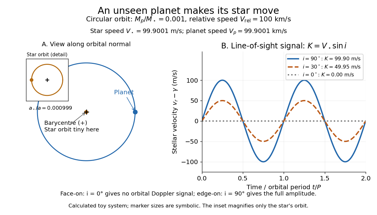
For a computed circular example, let $q=M_p/M_{\star }=0.001$ and choose a relative orbital speed $V_{\mathrm{rel}}=100\mathrm{km}{\mathrm{s}}^{-1}$: this is the speed of the planet relative to the star, not its speed about the astronomical barycenter. Conservation of momentum givesThe barycentric velocities point in opposite directions, so their speeds add to $V_{\mathrm{rel}}$. Here $e=0$ and $K=V_{\star }\sin i$: $K=99.9001\mathrm{m}{\mathrm{s}}^{-1}$ at $i=90^{\circ }$, $49.9500\mathrm{m}{\mathrm{s}}^{-1}$ at $i=30^{\circ }$, and zero at $i=0$. The star still orbits in the face-on case, but its orbital velocity has no line-of-sight component. The plotted circular signal is $v_r(t)-\gamma =K\sin (2\pi t/P)$ for a chosen phase origin and constant system velocity $\gamma$.

Methods of detecting exoplanets infer or resolve an exoplanet through its effects on the host star's light or through its own light. The observable determines what can be learned:

An exoplanet secondary eclipse measures the loss of the exoplanet's light when it passes behind its star, complementing exoplanet transit photometry. A detection method also selects which systems are easiest to find: deeper exoplanet transits favour larger radius ratios, and larger stellar radial-velocity semi-amplitudes favour more massive companions, shorter orbital periods, and larger $\sin i$. These preferences must be accounted for when inferring the underlying exoplanet population.

For a companion of negligible mass compared with its host, $M_p\sin i=K[P/(2\pi G){]}^{1/3}{M}_{\star }^{2/3}\sqrt{1-e^2}$. The observable supplies a projected mass; the minimum at a specified eccentricity occurs for an edge-on orbit. A exoplanet transit can constrain inclination, while low-inclination stars or brown dwarfs can otherwise mimic a lower-mass companion. The exact relation retains $(M_{\star }+M_p{)}^{2/3}$ in the denominator.

Adopt circular orbits, negligible planetary masses, spherical bodies, uniform stellar brightness and no transit dilution. Interpret the measured duration as the total duration of a circular planetary transit, from first to fourth contact, $T_{14}$. These conventions matter especially for the off-centre crossing: finite planet size cannot automatically be ignored there. Unknown orbital eccentricity or limb darkening would require further information to infer unique stellar radii.

First convert the apparent magnitude difference into a fractional exoplanet transit depth, rather than treating a milli-magnitude as a part in a thousand:Both crossings are non-grazing because their transit impact parameters satisfy $b<1-k$, so the full projected planetary disc can block the star. Equal depths determine equal radius ratios, not equal absolute planet radii.

For orbital inclination $i$ measured from the sky plane, $b=(a/R_{\star })\cos i$. Choosing mid-transit as orbital phase zero, the projected separation obeysAt first and fourth contact, $z/R_{\star }=1+k$. The full crossing duration therefore isFor the numerical scale use solar radius $R_{\odot }=6.957\times 10^8\mathrm{m}$ and nominal solar mass parameter $(GM{)}_{\odot }=1.3271244\times 10^{20}{\mathrm{m}}^3{\mathrm{s}}^{-2}$, with one day equal to $86400\mathrm{s}$. These are stated conversion choices, not additional measurements of the two systems.^[ref]

Kepler's third law gives $a=[G{M}_{\star }{P}^2/(4{\pi }^2){]}^{1/3}$. For a solar-mass, solar-radius host, this gives $a/R_{\odot }=12.3051$ at five days and $6.68023$ at two days. Substitution in the contact formula yieldsThe transit duration of a small planet instead takes both $k\to 0$ and $R_{\star }/a\ll 1$, giving $T\simeq P{R}_{\star }\sqrt{1-b^2}/(\pi a)$. It predicts $3.10\mathrm{h}$ and $1.37\mathrm{h}$, respectively. The difference is appreciable for B because the fractional change in its crossing chord is larger. Durations defined by mid-ingress to mid-egress or by second to third contact should not be silently equated with $T_{14}$.

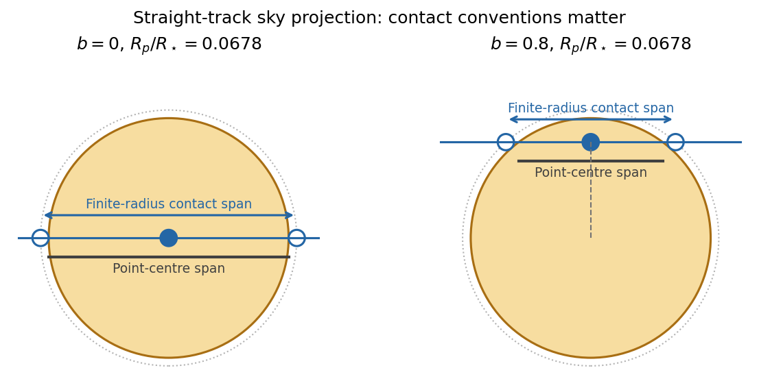
The original diagram uses a straight projected track to display the contact geometry; the duration formula above retains orbital curvature.

To infer the actual stellar radii, invert the contact formula before applying the supplied mass-radius scaling. Let $A=a/R_{\star }$ and $s=\sin (\pi T_{14}/P)$; thenThe measured durations imply $A_A=8.34661$ and $A_B=7.55743$. Normalize the stipulated constant mass-radius ratio to the Sun, so $M_{\star }/M_{\odot }=R_{\star }/R_{\odot }\equiv r_{\star }$. Kepler's third law then givesThus the stellar radius from transit duration and a linear mass-radius relation isThe same assumed scaling gives $M_A=1.79M_{\odot }$ and $M_B=0.831M_{\odot }$. A's longer crossing requires a lower mean stellar mass density, while B's shorter full-contact crossing requires a higher one. They are not both solar replicas under this model. Their planets have $R_{p,A}=0.1213R_{\odot }$ and $R_{p,B}=0.05633R_{\odot }$.

For a consistently applied point-planet approximation, the duration scales as $T\propto P^{1/3}{r}_{\star }^{2/3}\sqrt{1-b^2}$ and the inferred radii would instead be $R_A\simeq 1.98R_{\odot }$, $R_B\simeq 1.07R_{\odot }$. The latter is close to solar. Consequently the assertion of a substantial non-solar radius for B depends on which duration convention and finite-size approximation are intended. The contact-based values above use the measured depth rather than discarding it. If eccentric orbits are allowed, the transit speed introduces an additional factor depending on eccentricity and orientation, so the two durations alone cannot establish those radii uniquely.

For an outer coplanar planet around B, the common orbital inclination gives $b_2/b_B=a_2/a_B=(P_2/P_B{)}^{2/3}$. A point-planet centre must cross the stellar disc, requiring $b_2<1$. The usual coplanar transit limit is thereforeThis is a limiting value approached from below; a tangent path has no duration. For an outer planet of finite, unspecified radius ratio $k_2$, any overlap instead requires $b_2<1+k_2$, giving $P_2<P_B[(1+k_2)/b_B{]}^{3/2}$. If it had the same ratio $k_2=k$, that geometric limit would be $3.08$ days; requiring full overlap would give $2.52$ days. Because neither its radius nor a photometric detection threshold is supplied, no unique finite-size practical maximum period can be inferred beyond this conditional expression. The stellar radius cancels from the point-planet period-ratio bound.

For B's inner planet, a reflected-light planetary phase curve haswhere $A_g$ is geometric albedo and $\alpha$ is phase angle. Near exoplanet secondary eclipse the visible hemisphere is almost fully illuminated. Using the standard full-phase approximation and the contact-based $A_B$,The exact lost fraction of combined stellar and planetary light is $F_p/(F_{\star }+F_p)$, which changes the result negligibly at this contrast. The corresponding magnitude depth is about $0.0437$ milli-magnitudes. The circular orbit has the same impact distance at eclipse as at transit, and $b_B<1-k$, so the star can hide the entire planetary disc.

The inclination inferred for B is $83.92^{\circ }$, putting closest approach to full phase at $\alpha \simeq 6.08^{\circ }$. A fully precise prediction would therefore also require the reflected-light phase function, which the question does not specify; the boxed value uses $\Phi \simeq 1$. The consistent point-planet duration approximation yields about $56.7\mathrm{ppm}$ instead, through its different inferred $a/R_B$. It is important to keep the geometry used for the radius inference and the reflected-light calculation consistent.

Finally, the stellar radial-velocity semi-amplitude for a low-mass companion on a circular orbit isThe two stars' equal apparent magnitudes make a comparison at similar photon statistics plausible, though spectral-line widths, stellar variability and observing cadence can still differ. With the contact-based stellar estimates,If the planets have comparable mean densities, A is easier: their equal depth then gives $M_{p,A}/M_{p,B}\simeq (R_A/R_B{)}^3\simeq 9.99$, so $K_A/K_B\simeq 4.44$. The larger planetary mass outweighs A's longer orbital period and larger host mass. For equal planetary masses, B is easier by a factor $2.25$ in amplitude. The supplied transit data give planet radii, not masses, so the ranking is conditional on a planetary mass-radius assumption; a unique unconditional ranking would invent information.