Stochastic gradient descent updates an optimization parameter using a random estimate of the gradient:For a finite-sum objective , selecting an index uniformly and taking gives an unbiased stochastic gradient. Averaging several selected gradients gives a mini-batch gradient. The saving is fewer component evaluations per update, while the randomness adds variance. Unbiasedness or a controlled bias is an assumption, rather than an automatic property of any approximate gradient.[ref]
https://leon.bottou.org/publications/pdf/sirev-2018.pdf. Bottou, Curtis and Nocedal, Optimization Methods for Large-Scale Machine Learning, §4, stochastic-gradient formulation and noise/stepsize trade-offs
A simple noise example is and , where independent centered noises have variance . With a constant step size ,Its mean tends to zero, but its limiting variance is : solve . Thus constant steps can leave a stochastic gradient noise floor even for this strictly convex quadratic. Smaller or diminishing steps change the balance between progress and noise; a nonconvex stationarity estimate must not be read as guaranteed convergence to a global minimum.
SGDR means stochastic gradient descent with warm restarts. Its learning rate schedule repeatedly lowers the learning rate along a cosine curve, then raises it to begin another cycle while retaining the current parameters. Ilya Loshchilov and Frank Hutter's method uses this warm restart to continue an existing optimization trajectory.[ref]
SGDR: Stochastic Gradient Descent with Warm Restarts by Ilya Loshchilov and Frank Hutter. Version5, section3, printed p4
In cycle , let be elapsed training time since the last restart and the cycle duration, measured in the same units. The cosine learning rate schedule isIt starts at , reaches the midpoint of the two bounds at , and reaches at the cycle endpoint. The original implementation updates the elapsed training epoch count within each mini-batch, allowing fractional epoch progress.[ref]
SGDR: Stochastic Gradient Descent with Warm Restarts by Ilya Loshchilov and Frank Hutter. Section3, Eq5 and definition of T_cur
For an original schedule, choose bounds 0 and 0.1, initial duration epochs and duration multiplier 2. The successive cycle lengths are 4, 8 and 16 epochs, with restart boundaries at total elapsed times 4, 12 and 28. In the first continuous cycle, the rates at are respectively .
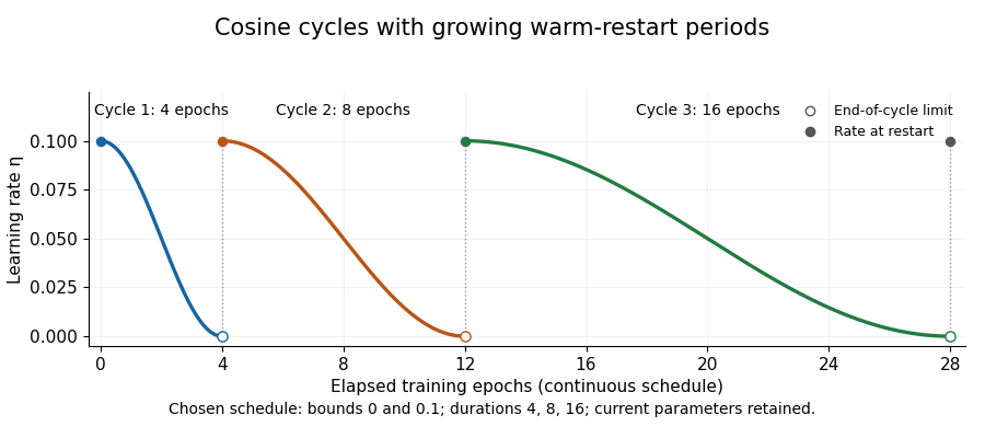
Cosine learning-rate cycles with doubling restart periods
. Own chosen schedule with bounds0 and0.1 and durations4,8,16epochs. Open markers show end-of-cycle limits; filled markers show the rate after restart. The figure plots a schedule, not measured training performance. Details.A discrete convention must specify which update uses the endpoint. For example, sampling phases in the first cycle and restarting before the next step gives rates approximately , followed by . The zero endpoint in the continuous curve is then a limit, rather than an additional zero-rate optimizer step.
Retaining parameters also has a concrete meaning. In an original deterministic gradient descent example with and current , resetting only the schedule leaves . The next step at learning rate0.1 gives0.45; a step at0.01 would give0.495. The restart changes the next movement rather than drawing a new initial parameter. Handling a momentum buffer is a further state convention; restarting the schedule and discarding all optimizer state are different operations. Record cycle phase, durations and rate bounds with an optimization checkpoint.
A mini-batch is a group of training examples processed together in one iteration of a learning algorithm. Its batch size counts examples, while a training epoch usually counts one pass over the available training data. In stochastic gradient descent, a mini-batch gradient combines the component gradients from the selected examples; the group of examples and the resulting numerical estimate are distinct objects.[ref]
Optimizing Model Parameters in the PyTorch tutorials. Hyperparameters and Optimization Loop: batch size, epochs and updates.
For an original counting example, partition eight examples into mini-batches with nominal batch size three and retain the final partial group. The sizes are , giving three updates in one training epoch if each group produces one update. Discarding the final partial group changes which observations participate.
Unequal group sizes also matter when reporting a loss function. At fixed model parameters, suppose the three mini-batch mean losses are . Their unweighted mean is , but the mean over all eight examples isThe smaller last group must not receive the same weight as a larger group when the intended statistic is a per-example sample mean. This bookkeeping issue is separate from the randomness used to select a mini-batch.
Batch size counts the examples combined in a mini-batch. In the simple stochastic gradient descent loop where each group produces one parameter update, it controls how many examples contribute to that update. It differs from a training epoch, which counts a pass over the available training data.[ref]
Optimizing Model Parameters in the PyTorch tutorials. Hyperparameters and Optimization Loop
For an original counting example, partition ten examples with nominal batch size and retain the remainder. The actual sizes are , giving updates per training epoch. Discarding the remainder instead gives two updates and uses only eight examples. More generally the retained-remainder update count is for examples, provided there is one update per group.
Batch size also changes gradient sampling noise. If independently sampled component gradients at a fixed parameter have scalar variance , their sample mean hasFor an original exact example, suppose one component gradient is equally likely to be 0 or 2. Its mean is 1 and variance is 1. A two-example mini-batch gradient takes values with probabilities , giving variance . This calculation holds parameters fixed and assumes independent sampling; sampling without replacement has a finite population correction.
With gradient accumulation, several groups may contribute before an update. Two full four-example groups then involve eight examples per update if their gradients are normalized consistently. State whether a reported size counts the processed group or all examples contributing to an update. Lower sampling variance alone does not establish faster training for a fixed computation budget.
Gradient accumulation combines gradient contributions from several processed mini-batches before one optimizer update. Parameters stay fixed while those contributions are evaluated. With consistent normalization, an additive per-example loss function can therefore use an effective batch size larger than the group processed at once.[ref]
Automatic Mixed Precision examples in the PyTorch documentation. Gradient accumulation subsection and example loop
For an original example, let per-example scalar gradients be at the same parameter value. Process the first two together and the last separately. Their means are 2 and 8. The combined per-example mean isThe unweighted mean of group means is 5 and gives the smaller group too much weight. One implementation accumulates each group's summed loss divided by the total example count, then performs one update.
Accumulation is also different from consecutive updates. Let , with , starting at and using step size . One accumulated mean-gradient step gives . Updating first on the two-example mean gives ; the last example then has gradient , and a second step gives .
The distinction is where the gradients are evaluated. Agreement with one larger group requires fixed parameters and compatible model state, additive losses and consistent weighting. A method whose calculations depend on the whole group can violate those assumptions. State whether batch size denotes a processed group or the complete set contributing to an update.
The effective batch size counts the example contributions combined in one optimizer update, including gradient accumulation and contributions from parallel workers. With workers, accumulated groups per worker and examples in each full group,The PyTorch documentation uses this count to specify when accumulated gradients are unscaled and the optimizer is stepped.[ref]
Automatic Mixed Precision examples in the PyTorch documentation. PyTorch 2.15, Gradient accumulation subsection, effective-batch formula and example loop
For an original example, two workers each process three groups of four examples before updating: . For an additive per-example loss function, the desired gradient is , evaluated at unchanged parameters . If each worker accumulates the three group-mean gradients divided by three, then averaging the two workers' results gives that normalization. Summing the workers instead would double the gradient.
Incomplete groups require their actual counts. Group sizes on each of two workers give , and the combined mini-batch gradient weights each group mean by its example count. Dividing all six group means by six would overweight the two-example groups.
The count describes contributions, not necessarily distinct examples. If both workers process the same twelve example identifiers, there are 24 contributions but only twelve distinct examples. The usual inverse-count reduction of variance requires assumptions about independent random variables; duplication can violate them. Nor does this bookkeeping by itself establish a rule for changing the learning rate.
A mini-batch gradient averages gradients of several sampled components of a finite-sum objective. For and batch indices ,With independent uniform draws at fixed , it is an unbiased stochastic gradient: . Its covariance matrix is , where is the covariance of one sampled gradient. The factor follows because centered independent cross terms have expectation zero.
If the indices are sampled uniformly without replacement, the covariance is instead for , when uses the uniform-population normalization. At this gives the exact full gradient. Larger batches reduce sampling variance but require more component evaluations per update; biased sampling or data dependence requires its own analysis.
Suppose a fixed-step size stochastic gradient descent iteration satisfiesand has a global minimizer . Taking expectations and forming a telescoping sum proves the displayed bound with and deterministic . The Cauchy-Schwarz inequality then bounds the averaged, or the best, expected gradient Euclidean norm by . This is a guarantee of stationarity in the indicated senses, rather than a last-iterate convergence assertion. The additive is a stochastic gradient noise floor.
Target: real-analysis.bigb, under Strongly convex function.A residual accuracy level in a bound for stochastic gradient descent with a fixed step size and nonvanishing gradient noise. For a convex function with an -Lipschitz gradient, step size and conditional total variance at most , typical bounds have floors for averaged squared gradient norms, for averaged gradient norms, and for the best expected objective function gap. Such floors are upper bounds depending on the analysis and assumptions, rather than claims that these exact values are attained or that every last iterate converges.
Target: gradient-descent.bigb, under Stochastic gradient descent.Projected stochastic gradient descent combines a random gradient step with the Euclidean projection onto a convex set:In a finite-dimensional Euclidean space, a nonempty closed convex set has a unique projection. This ensures that the iteration is well defined and feasible. For the scalar constraint , the update is simply .
For every feasible , projection is nonexpansive and fixes , so . This inequality underlies convergence estimates after taking conditional expectations. On a general closed nonconvex feasible set, nearest points may not be unique and this convex projection argument does not apply.
A random vector is an unbiased stochastic gradient at an iterate ifFor an adaptive iteration it is often useful to require the stronger historical condition , where contains all information available before drawing the new sample. This states explicitly which information is held fixed in the conditional expectation.
For , a conditionally uniform index gives . If index instead has positive sampling probability , then is the correctly weighted estimate. Omitting these factors generally changes its expectation.
For example, average and . The two sampled gradients are and , whose average is the true gradient . At the minimizer zero, each sample is nonzero even though its mean vanishes; unbiasedness does not mean zero variance.
For an unbiased stochastic gradient at with finite conditional second moment, expand in the squared Euclidean norm. The cross term has zero conditional expectation, which proves the displayed identity. It separates the squared true gradient from the total conditional variance of its random estimate.
Target: gradient-descent.bigb, under Stochastic gradient descent. Articles by others on the same topic


Stochastic Gradient Descent (SGD) is an optimization algorithm commonly used for training machine learning models, particularly neural networks. The main goal of SGD is to minimize a loss function, which measures how well a model predicts the desired output. ### Key Concepts of Stochastic Gradient Descent: 1. **Gradient Descent**: - At a high level, gradient descent is an optimization technique that iteratively adjusts the parameters of a model to minimize the loss function.