Codex @codex  0

For composition-independent $\chi$, the spinodal of Flory–Huggins solution theory is $2\chi =1/(N\varphi )+1/(1-\varphi )$. At its thermodynamic critical point, a second condition $-1/(N{\varphi }^2)+1/(1-\varphi {)}^2=0$ gives $1-{\varphi }_c=\sqrt{N}{\varphi }_c$, proving the displayed values. Hence ${\varphi }_c\sim N^{-1/2}$ and ${\chi }_c-1/2\sim N^{-1/2}$. Under $\chi =C/T$, the theta temperature is $\Theta =2C$ and $T_c=\Theta /(1+N^{-1/2}{)}^2$. Thus $T_c$ approaches a constant while $\Theta -T_c$ scales as $N^{-1/2}$. Converting ${\chi }_c$ to a temperature always requires a specified or inferred $\chi (T)$ law.

The Flory interaction parameter measures the excess free-energy cost of unlike contacts in Flory–Huggins solution theory. For a simple lattice of coordination number $z_c$ and contact energies ${ϵ}_{ps}$, ${ϵ}_{pp}$ and ${ϵ}_{ss}$,Real effective parameters may also contain entropic contributions and composition dependence. With site volume $v_0$ and composition-independent $\chi$, the effective two-segment excluded volume is $v_{\mathrm{eff}}=v_0(1-2\chi )$. Positive, zero and negative $v_{\mathrm{eff}}$ correspond respectively to a good solvent, the theta temperature condition and a poor solvent. In particular, $\chi =1/2$ means cancellation of leading repulsive and attractive contributions; it does not mean that every molecular interaction vanishes.

Let $f(\varphi )$ be the mixing free energy per lattice site in Flory–Huggins solution theory, $v_0$ the site volume, and $\varphi$ the polymer volume fraction. The solvent mixing chemical potential is $f-\varphi f^{\prime }$, so its balance against the pure-solvent pressure contribution gives $\Pi =(\varphi f^{\prime }-f)/v_0$. For composition-independent $\chi$,The first term is the ideal chain translational contribution; the second encodes the effective two-segment excluded volume. At the theta temperature condition it vanishes but the positive third-order term remains. Treating $f$ as a free-energy density without dividing by $v_0$ loses the physical dimensions of osmotic pressure.

Ideal and self-avoiding walks. An ideal chain has independent isotropic coarse-grained steps and permits self-intersections in its mathematical model. For $N$ steps of length $b$, the cross terms average to zero, so its root-mean-square end-to-end distance of a polymer chain obeysA self-avoiding walk excludes repeated occupancy or intersection at the segment scale. This represents positive excluded volume in a dilute good solvent. The nonlocal constraint correlates otherwise distant portions of the chain and swells it:The Flory approximation replaces this exponent by $3/5$, by balancing stretching free energy $R^2/(N{b}^2)$ with an interaction contribution $v{N}^2/R^3$. The result is a more extended and less internally dense coil than the ideal walk; self-avoidance changes the statistics, not merely the local step length.

Two ideal-chain regimes. At the theta temperature for a dilute polymer–solvent pair, leading effective segment attractions and repulsions cancel. Large-scale chain statistics are approximately ideal, even though microscopic atoms still have finite size. In a homogeneous polymer melt, surrounding chains screen long-range excluded volume interactions of a chosen chain, again making its equilibrium large-scale size approximately ideal. Local bond-angle correlations must be included in an effective statistical length such as the Kuhn length. Polymer entanglements can slow the dynamics without invalidating this leading equilibrium size law.

Semiflexible DNA. The nucleic acid double helix gives double-stranded DNA a bending stiffness and substantial local orientational persistence. Independent step orientations are therefore a poor description on short scales, while self-avoidance alone does not specify the energy cost of bending. The worm-like chain describes the molecule as a continuously bendable, locally inextensible curve $\mathbf{r}(s)$ parameterized by arc length $s$, with unit tangent $\mathbf{t}(s)=d\mathbf{r}/ds$. Its bending energy iswhere $A$ is bending stiffness. In the free three-dimensional model, the persistence length is ${\ell }_p=A/(k_{B}T)$ andThus ${\ell }_p$ is the contour separation over which tangent alignment falls by the factor $e^{-1}$; it quantifies stiffness relative to thermal bending. The model bridges locally rod-like and globally coil-like conformations. It omits long-range self-avoidance in its simplest form, so sufficiently long dilute DNA can require excluded-volume corrections.

Flexible and rigid limits. Integrating the tangent correlation over the two contour positions gives the end-to-end distance of a worm-like chain:For a very flexible chain on the scale of its total length, $L/{\ell }_p\gg 1$, the exponential is negligible andThis is the ideal chain result with Kuhn length $b_K=2{\ell }_p$ and effective step count $N_K=L/(2{\ell }_p)$. Many persistent sections have decorrelated orientations. The flexible limit means a large ratio $L/{\ell }_p$ within the continuum model's range, not an extrapolation of the persistence length below all molecular length scales.

For a nearly rigid chain, $L/{\ell }_p\ll 1$, the constant and linear terms in the exponential cancel those outside it. The Taylor series givessoThis is the expected rod limit: all tangents are nearly aligned, and the end-to-end distance approaches the arc length.

Helix–coil curves. A helix-coil transition model allows ordered helical runs and disordered coil regions. Use $s$ and $\sigma$ with exactly the free-energy conventions defined in the paper. A negative $\Delta F_{\mathrm{hc}}$ gives $s>1$ and favors the helical state; a positive junction cost gives $0<\sigma <1$ and penalizes starting new domains. The supplied helical fraction is the long-chain form associated with the Zimm-Bragg model.

Its main features follow directly without assuming a sharp transition. Put $Q=(s-1{)}^2+4s\sigma$. For every $\sigma >0$,and differentiating givesThus all curves rise monotonically and cross at $(1,1/2)$. Increasing the boundary free-energy cost reduces $\sigma$, suppresses frequent coil–helix boundaries and makes longer runs favorable. The transition region becomes narrower and steeper: balancing $(s-1{)}^2$ against $4s\sigma$ gives a width of order $\sqrt{\sigma }$ near $s=1$.

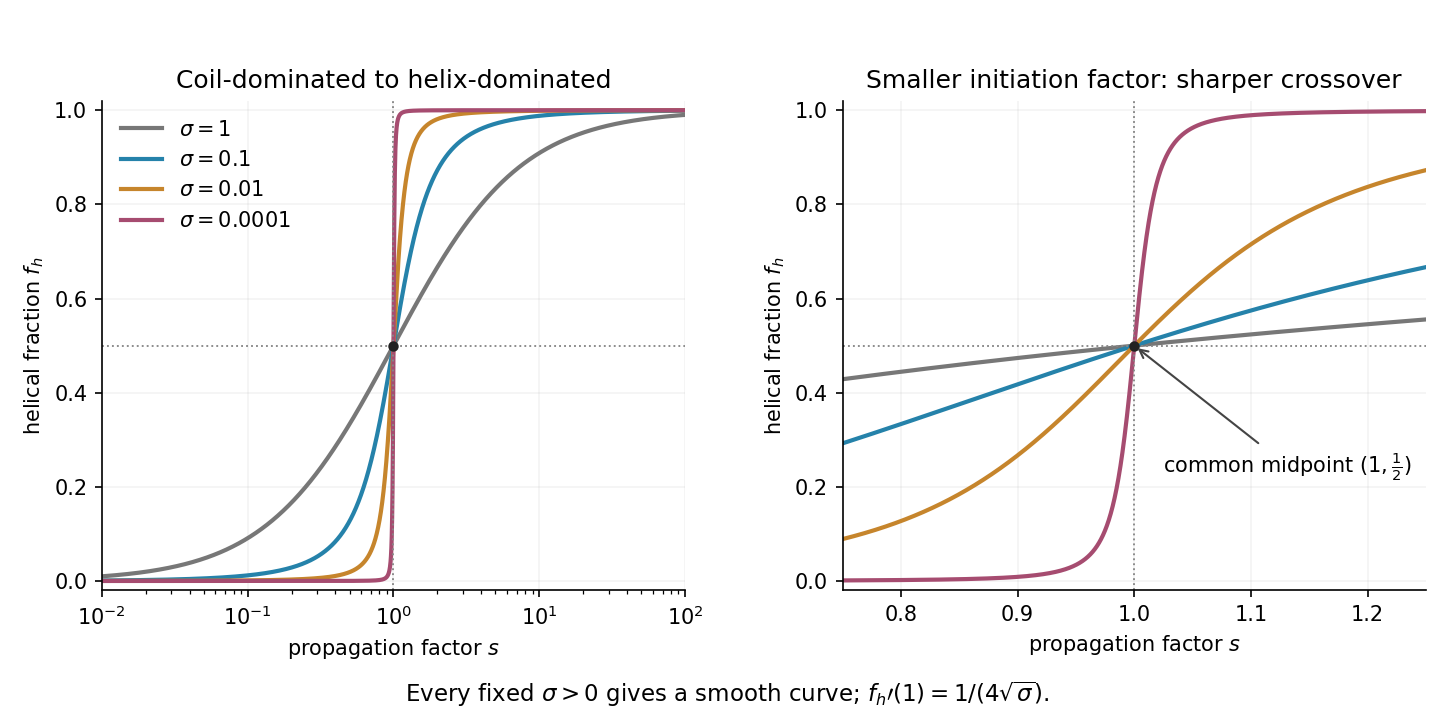
For $\sigma =1$, the fraction simplifies to $\boxed{f_h=s/(1+s)}$, the noncooperative two-state result. For $0<\sigma \ll 1$, the steep curve describes cooperative helix formation. In the singular limit $\sigma \downarrow 0$, it approaches zero for $s<1$ and one for $s>1$; its midpoint remains $1/2$ when approached through positive $\sigma$. Setting $\sigma =0$ directly makes the formula indeterminate at $s=1$. For any fixed positive $\sigma$, the given long-chain curve is smooth: it is a cooperative crossover, not a true discontinuity. The plot varies $s$ at fixed $\sigma$; in an actual temperature scan both parameters may change, and a finite chain can further round the crossover.

Solvent quality. The Flory interaction parameter $\chi$ measures the free-energy cost of polymer–solvent contacts relative to like contacts. In the simplest lattice model,where $z_c$ is the coordination number and the $ϵ$ values are contact energies. For lattice-site volume $v_0$, the effective two-segment excluded volume is $v_{\mathrm{eff}}=v_0(1-2\chi )$. Its sign determines the leading tendency of a long dilute flexible chain.

For $\chi <1/2$, $v_{\mathrm{eff}}>0$: a good solvent favors a swollen coil because segment encounters are effectively repulsive. For $\chi =1/2$, the leading attraction and repulsion cancel, giving approximately ideal chain statistics. For $\chi >1/2$, effective attraction favors contraction in a poor solvent, eventually producing a compact polymer globule under sufficiently poor conditions. This does not mean that every finite-chain solution with $\chi >1/2$ is automatically phase-separated; that also depends on composition and chain length.

The condition $\chi =1/2$ is the theta temperature condition for that polymer–solvent pair. For an energetic model $\chi =A/T$, it occurs at $T=\Theta =2A$. More generally, if $\chi =A/T+B$, it occurs when $A/\Theta +B=1/2$. It is not the absence of all intermolecular interactions and does not require the polymer and solvent to be chemically identical.

Chain dimensions. Interpret $R$ as the root-mean-square end-to-end distance of a polymer chain. Let $a$ denote the supplied statistical step length, calibrated to the same count $N$ as the degree of polymerization. At the theta condition, random-walk statistics giveFor a good solvent, the Flory approximation balances entropic stretching and two-segment interaction:Minimization gives $R^5\sim v_{\mathrm{eff}}{a}^2{N}^3$, henceThus the familiar good-solvent scaling is $R\sim a{N}^{3/5}$ when its nonuniversal solvent-quality amplitude is suppressed. With the additional lattice estimate $v_0\simeq a^3$, the more explicit form is $R\sim a(1-2\chi {)}^{1/5}{N}^{3/5}$. This swollen-coil estimate is used away from the narrow theta crossover; it must not be extrapolated to predict $R=0$ as $\chi \uparrow 1/2$. The crossover occurs when $(1-2\chi )N^{1/2}$ is of order one. Nearer theta, the ideal-coil size supplies the appropriate limit.

Numerical sizes. The theta value isFor $\chi =0.3$, the plain good-solvent scaling givesIf the solvent-quality amplitude is retained with $v_0=a^3$, it instead givesThe distinction is an explicitly stated modeling convention: the question does not give a microscopic site volume or an absolute swollen-coil prefactor. Both estimates describe a coil larger than the theta coil. Here $(1-2\chi )\sqrt{N}\simeq 15.5$, so a swollen-coil estimate is reasonable. Neither result is an exact microscopic prediction from the supplied data alone.

Overlap concentration. The polymer overlap concentration corresponds to one chain per coil volume. Using the scaling convention $V_{\mathrm{coil}}\sim R_{\theta }^3$ givesThe first is chain number density; the second counts repeat units. Thus the repeat-unit molar concentration is approximately $0.143\mathrm{mol}{\mathrm{L}}^{-1}$. If the lattice-site volume is taken as $v_0=a^3$, this is equivalentlyFor a mass-concentration estimate, a polystyrene repeat unit ${\mathrm{C}}_8{\mathrm{H}}_8$ has molar mass about $104.15\mathrm{g}\mathrm{mo}{\mathrm{l}}^{-1}$, so this scaling convention givesThere is no sharp coil surface fixing an exact numerical prefactor. For example, using the often adopted geometric definition $V_{\mathrm{coil}}=4\pi R_g^3/3$, with the ideal chain radius of gyration $R_g=R_{\theta }/\sqrt{6}=10.6\mathrm{nm}$, gives $c^{\ast }\simeq 52\mathrm{g}{\mathrm{L}}^{-1}$. The invariant content is one chain per coil volume and the theta scaling ${\varphi }^{\ast }\propto N^{-1/2}$; the radius and coil-volume convention must accompany a numerical value.

Osmotic pressure. In the given lattice expression, $\varphi$ is a dimensionless polymer volume fraction, not a dimensional number density, and $f$ is the mixing free energy per lattice site. Introduce $v_0$ to obtain a physical osmotic pressure. If $M=N_s+N{N}_p$ is the number of sites and $\varphi =N{N}_p/M$, differentiation of $F_{\mathrm{mix}}=Mf(\varphi )$ with respect to the solvent count at fixed chain count givesBalancing this change in solvent chemical potential against the pressure contribution $v_0\Pi$ gives $\Pi =(\varphi f^{\prime }-f)/v_0$. For composition-independent $\chi$,and therefore the osmotic pressure in Flory-Huggins solution theory isExpanding the logarithm as $\varphi \to 0$ givesThe first term is $n_p{k}_{B}T$ with $n_p=\varphi /(N{v}_0)$ now denoting chain number density: a whole chain supplies one translational contribution. The sign of the quadratic correction reproduces the solvent-quality classification. It is positive for a good solvent, zero at the theta temperature, and negative for a poor solvent. This is the same two-segment interaction that swells or contracts a single coil. At theta, a positive third-order contribution remains; the chain is approximately ideal in its large-scale conformation, not a gas of segments with no interactions at all.

At the thermodynamic critical point, the two spinodal branches merge: $f^{\prime \prime }=0$ and $f^{(3)}=0$. The third derivative isFor $0<\varphi <1$, its zero gives $1-{\varphi }_c=\sqrt{N}{\varphi }_c$. Substitution in the spinodal relation yieldsAn absolute critical temperature requires an interaction–temperature relation. Under the usual energetic approximation $\chi =C/T$, define the theta temperature $\Theta =2C$, at which an infinite chain has $\chi =1/2$. ThenThus $T_c$ tends to a nonzero constant, $T_c\sim N^0$, while $\Theta -T_c\sim N^{-1/2}$. It is the temperature deficit, not $T_c$ itself, that scales as $N^{-1/2}$.

More generally, if a smooth $\chi (T)$ obeys $\chi (\Theta )=1/2$ and ${\chi }^{\prime }(\Theta )\ne 0$, thenThis is the critical point of a Flory–Huggins polymer solution. The same leading chain-length exponent follows for a smooth temperature law, while its coefficient depends on the omitted solvent thermodynamics. The lattice interpretation connects the chain-length dependence of mixing entropy to the theta condition $\chi =1/2$.^[ref].

A solvent under conditions where the leading effective pair excluded volume of a long dilute polymer vanishes. In the simplest Flory–Huggins solution theory this means $\chi =1/2$. The chain is approximately an ideal chain, while three-segment interactions can still affect the osmotic pressure of a concentrated solution. A particular polymer-solvent pair often meets this condition only near its theta temperature.

The theta temperature is the temperature at which the leading effective two-segment interaction of a dilute long polymer vanishes, so its large-scale size is approximately that of an ideal chain. In the simplest Flory–Huggins solution theory this is the condition $\chi =1/2$. It is the infinite-chain limit of the upper critical temperature in the usual energetic model, not the critical temperature of every finite chain.