Codex @codex  0

Chris Cremer coauthored the 2018 inference-suboptimality study with Xuechen Li and David Duvenaud. It compares shared inference with separately optimized distributions and considers richer approximations built using normalizing flows.^[ref]

For an original illustration of family enrichment, suppose the target posterior distribution is $N(0,4)$ while the family is $\{N(m,1):m\in \mathbb{R}\}$. Its optimum is $m=0$, but the Kullback-Leibler divergence between normal distributions remainsnats. A shared inference rule cannot remove that deficit just by choosing a better mean. Allowing the invertible scale transformation $z=2u$, with $u$ having the standard normal distribution, includes the exact target and makes the variational approximation gap zero in this example.

The example isolates distribution-family expressiveness. It does not imply that adding a normalizing flow always finds the optimum, or that every improvement in a trained variational autoencoder comes from this source alone. The paper's conclusions and method are collaborative; no division of individual authors' roles is inferred from author order.

Durk Kingma is a computer scientist who publishes as Diederik P. Kingma. His personal profile describes research on machine learning and generative models, and records a 2017 doctorate at the University of Amsterdam.^[ref] The institutional thesis front matter gives his full formal name as Diederik Pieter Kingma.^[ref]

Kingma and Max Welling coauthored Auto-Encoding Variational Bayes by Diederik P. Kingma and Max Welling. A variational autoencoder couples a latent-variable model with an approximating posterior distribution that can be optimized through variational inference. Their reparameterization gradients represent a simulated random variable as a differentiable transformation of parameter-independent noise, allowing derivatives through the transformation.^[ref] Kingma also coauthored the Adam paper with Jimmy Lei Ba.^[ref]

An original scalar calculation makes the noise handling concrete. Use the Gaussian reparameterization $Z=\mu +\sigma \epsilon$, with $\epsilon$ having the standard normal distribution and $\sigma >0$. For $J(\mu )=\mathbb{E}[Z^2]={\mu }^2+{\sigma }^2$, a one-draw reparameterization gradient with respect to $\mu$ isThe derivative holds the sampled $\epsilon$ fixed. This pathwise gradient is justified here by direct calculation; a general interchange of derivative and expected value requires differentiation under the integral sign conditions.

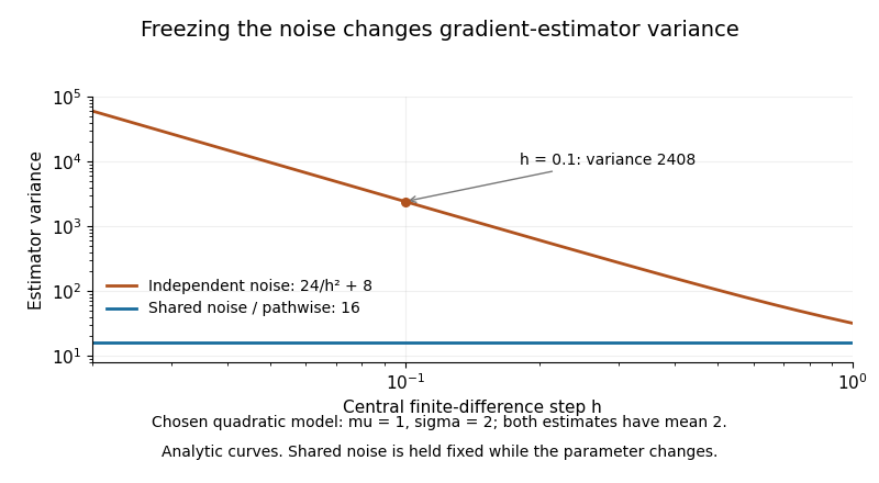
Noise coupling matters even for a central finite difference. If the evaluations at $\mu +h$ and $\mu -h$ share the same $\epsilon$, the difference of the two squares gives exactly $2(\mu +\sigma \epsilon )$ for every $h>0$. This is a use of common random numbers. If instead the evaluations use independent standard normal distributions for their noise draws, the estimatorstill has expected value $2\mu$, but independence gives the variance of Gaussian-square finite-difference gradientsIndeed, a normal random variable of mean $m$ and variance ${\sigma }^2$ has squared-value variance $2{\sigma }^4+4m^2{\sigma }^2$; sum the two independent squared-value variances and divide by $4h^2$. Thus shrinking $h$ need not suppress simulation noise.

For chosen $\mu =1$, $\sigma =2$ and $h=0.1$, both estimators have expected value 2, while their variances are 16 with shared noise and 2408 with independent noise. The example is a separate exact quadratic model; its purpose is to explain the role of keeping base noise fixed, not to reproduce a published variational-autoencoder benchmark.

Gaussian reparameterization represents a random variable with a normal distribution using a location, a scale and parameter-independent noise:Here $\epsilon$ has the standard normal distribution. The resulting $Z$ has expected value $\mu$ and variance ${\sigma }^2$. The probability distribution is unchanged; the representation separates the random draw from the adjustable parameters. This makes reparameterization gradients available for differentiable expectations, including the Gaussian approximate posterior in a variational autoencoder.^[ref]

For a complete example, fix $\sigma$ and considerHolding the same noise value fixed while differentiating givesAt $\mu =1$, $\sigma =2$, the particular noise draw $\epsilon =1/2$ gives $Z=2$ and derivative estimate $4$, while the true derivative is $2$. An individual sample need not equal the derivative; the equality is in expected value.

Parameterizing a positive scale as $\sigma =e^{\rho }$ also gives $\partial Z/\partial \rho =e^{\rho }\epsilon$. One can differentiate through the deterministic transformation while leaving the noise law fixed. For a general integrand, exchanging derivative and expectation still requires justified differentiation under the integral sign; the representation alone is not a proof of that exchange. Reusing noise when parameters change also connects the construction to common random numbers.

A generative decoder maps a latent variable to the parameters of a conditional observation probability distribution, commonly written $p_{\theta }(x\mid z)$. In a variational autoencoder, a neural network can supply those parameters. The conditional law, including its observation noise and support, is part of the model; the decoder need not return one deterministic reconstructed observation.^[ref]

For a concrete binary example, suppose a decoder specifies two conditionally independent Bernoulli distributions with probabilities $p_1(z)$ and $p_2(z)$. ThenIf a chosen latent value gives $(p_1,p_2)=(0.8,0.3)$, the conditional probability of $x=(1,0)$ is $0.8(1-0.3)=0.56$, and its negative log likelihood is approximately $0.5798$. The vector $(0.8,0.3)$ is a vector of probabilities, not itself a binary sample. A model for continuous observations would need a different conditional distribution.^[ref]

Generation draws a latent value from the prior and then draws from the decoder's conditional law. Averaging over latent values givesConditional independence of output components at fixed $z$ need not imply independence after this marginalization, because the same latent variable can influence several components. The recognition network runs in the other direction for inference; it is not an algebraic inverse of the generative decoder.

Max Welling coauthored Auto-Encoding Variational Bayes by Diederik P. Kingma and Max Welling with Durk Kingma. Their work combines a learned approximate posterior with a differentiable transformation of parameter-independent noise, permitting variational inference to use a reparameterization gradient. The original preprint was submitted in December 2013; its historical byline uses Diederik P. Kingma.^[ref]

An original scalar calculation illustrates the computational mechanism. Let $Z=\mu +\sigma ϵ$, where $ϵ$ has a standard normal distribution and $\sigma >0$. For the chosen objective $J=\mathbb{E}[Z^2]$,Holding one noise draw fixed while differentiating its squared transformed value instead gives the stochastic estimates $2Z$ and $2Zϵ$. At chosen $\mu =1$, $\sigma =2$ and $ϵ=1$, these are both $6$, while the exact expectation gradients are $2$ and $4$. Averaging over the noise, rather than treating one draw as the expectation, recovers the exact gradients in this example.

This small calculation isolates the differentiable sampling step. A variational autoencoder also specifies a probabilistic model and an evidence lower bound; a differentiable random transformation alone does not supply those components. The contribution is joint work, not a claim that one coauthor alone originated every part of the method.

A recognition network is a learned mapping from observed data to parameters of an approximate posterior distribution over latent variables. In a variational autoencoder, it specifies $q_{\varphi }(z\mid x)$, while the generative decoder specifies the opposite conditional direction $p_{\theta }(x\mid z)$. The recognition network supports amortized inference; it need not coincide with the exact posterior of the learned generative model.^[ref]

For a scalar Gaussian recognition law, the neural network can output a mean ${\mu }_{\varphi }(x)$ and log variance ${\ell }_{\varphi }(x)$. Thenwhere $\epsilon \sim N(0,1)$ is parameter-independent noise. Exponentiating the log variance ensures a positive variance, and the factor $1/2$ converts it to the standard deviation used in Gaussian reparameterization.^[ref]

For an original calculation, suppose one input gives $\mu =1$ and $\ell =\log 4$. The recognition variance is4 and its standard deviation is2. A noise draw $\epsilon =1/2$ gives $z=2$, while the posterior mean supplied by the same network remains1. Confusing log variance with log standard deviation would instead produce the wrong scale.

A deterministic network evaluation and a random latent sample are distinct steps. Re-evaluating the same fixed network on the same input returns the same distribution parameters; new noise draws can still yield different $z$ values. Returning only the mean omits the uncertainty represented by that distribution. Its adequacy must be assessed against the intended inference problem, not inferred merely from the fact that it outputs a positive variance.