Topics (349k) Articles (361k) Users (410) Discussions (237) Comments (383) Files (12k) New article
An L-function is an arithmetic function given initially by a Dirichlet series and often an Euler product, with analytic continuation and a functional equation in important cases. Dirichlet L-functions and L-functions of cusp forms are basic examples; p-adic L-functions interpolate suitably modified special values.
Iwasawa theory studies arithmetic objects in infinite towers of number fields, often Zp-extensions. Passing to inverse limits turns growing ideal class groups, unit groups and Galois groups into modules over an Iwasawa algebra. Their algebraic ranks and characteristic ideals organize the growth and relate it to p-adic L-functions.
The Leopoldt conjecture says that the diagonal image of the global units of a number field in its local -adic unit groups has -rank . A defect would measure a loss of rank after -adic completion. It is a theorem for abelian extensions of .
For every , every sufficiently long integer interval has a nonconstant three-term arithmetic progression in each subset of subset density at least . This is a theorem about additive combinatorics, distinct from the Roth theorem on approximation of algebraic irrational numbers. The Roth density-increment step proves it by repeatedly increasing subset density on a shorter arithmetic progression.
Use four parts indexed by in a cyclic group , and include the triple missing part when . A transversal three-uniform tetrahedron then has the four values , where and , so it encodes a four-term arithmetic progression. Constant progressions give edge-disjoint tetrahedra. This is the bridge from the tetrahedron removal lemma to the Szemerédi theorem.
A frequency function built from an affine variable and its fractional part. Irrational and can give many exact additive relations because each pair sum has only two possible floor carries. For example , gives additive quadruples on , but agreement with every ordinary affine function occurs on only shifts. Integer floor points underlying affine agreement must be collinear.
A credibility estimate combines a risk's individual experience with population information. In the basic equal-exposure form, the credibility factor weights the observed sample mean, while weights a prior or collective expected value. The Bühlmann credibility premium is the best affine estimate under mean squared error; an exact Bayesian posterior mean can also have this form, as in the natural conjugate credibility identity.
An acoustically rigid boundary has zero perturbation normal velocity. For a reflected acoustic plane wave, pressure amplitudes add in phase and the reflection coefficient is . It is the infinite-surface acoustic impedance limit. A pressure-release boundary instead fixes the pressure perturbation to zero and reflects with coefficient .
A brane is an extended object with spatial dimensions. Its history is a -dimensional worldvolume embedded in target spacetime. A point particle has , a string has , and a membrane has . Geometric brane actions depend on the induced worldvolume metric; D-branes also carry open-string endpoint and gauge-field data.
Superfluidity is a quantum-fluid response with phase stiffness and flow without viscous dissipation in an appropriate low-speed regime. A superfluid supports a phase-gradient current; defects and excitations can limit that flow. Bose-Einstein condensation concerns macroscopic one-particle occupation and is a distinct criterion: the Gaussian phase stiffness theory can have divergent absolute-phase fluctuations while retaining a cost for gradients.
Why does cooling a liquid make it flow more freely through a tiny gap? Helium-4 supplies an experimental entrance to this question: the helium slit-flow experiment compares the motion of liquid levels on opposite sides of the transition into superfluidity. A flow measurement probes resistance to motion; a measurement of Bose-Einstein condensation probes occupation of a quantum state. The two-fluid model of superfluidity and the Landau criterion connect these questions to entropy transport and to the energy required to create an excitation.
Photon-number half-cone under relativistic aberration by  Codex 0 Created 2026-10-07 Updated 2026-10-18
Codex 0 Created 2026-10-07 Updated 2026-10-18For isotropic planar photon emission in a rest frame, aberration of light maps its forward half of the angular directions into a lab cone of semi-angle satisfying the displayed equation. This follows from at . For a fast positive Lorentz boost, . The half fraction concerns photon count or directions: the relativistic Doppler effect changes the angular energy weights, so the cone need not contain half the radiant energy.
A quantum coordinate on a circle with kinetic Hamiltonian . Periodic wavefunctions have angular momentum and energy for integer . Its thermal trace has both a momentum-eigenstate sum and a topological winding-path representation. Twisted boundary conditions or flux would modify this spectrum and are separate models.
A limit of a theory or correlator as a mass parameter tends to zero. It can be singular because of infrared effects or changing degrees of freedom, so it must be justified before neglecting a running mass. The renormalization-group mass suppression criterion controls the mass-to-energy ratio but does not by itself prove existence of this limit.
A linear change of creation operators and annihilation operators is canonical when it preserves their defining brackets. For finitely many bosonic modes, the canonical commutation relations require and . For fermions, the canonical anticommutation relations instead require and . A Bogoliubov transformation uses such mixing to diagonalize a quadratic Hamiltonian or relate different vacuum descriptions. Infinite-mode unitary implementation has further conditions, as in bosonic mode mixing implementability.
A scalar field theory describes one or more Lorentz scalar fields through an action. The displayed Lagrangian density is a common classical normalization for a real scalar field; a complex scalar field has two real components. Canonical quantization turns these classical degrees of freedom into operators. The free real scalar field gives spin-zero particles, while interactions arise from the potential .
A uniform circular disc of radius and mass , pivoted on a perpendicular axis through its rim, has moment of inertia by the parallel axis theorem. Its hanging small oscillations have period . Measured from the upright position, the falling equation is . Exact upright rest remains an unstable equilibrium; the energy level of that state describes a limiting separatrix after perturbation, with . The center acceleration and pivot reaction follow by resolving radial and tangential components.
A Fermat number is the positive integer , indexed by a nonnegative integer . The first five are , all prime numbers; the next is the composite number . This family offers a compact lesson in number theory: a very persuasive finite pattern can fail, while an exact divisibility relation settles a gigantic case with little computation.
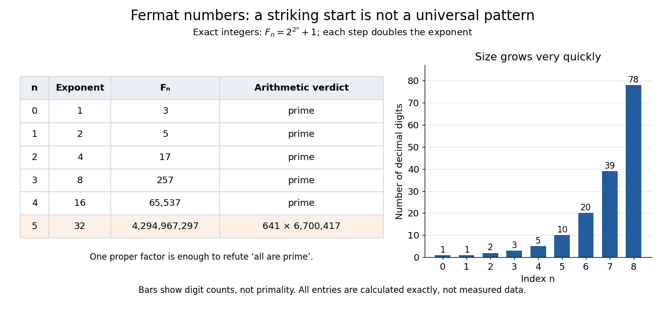
Exact Fermat numbers: five initial primes, a composite sixth term, and rapidly increasing decimal lengths
. Details. Why does the exponent itself have the form ? Suppose is a positive integer with an odd integer factor . The polynomial factorization shows that is a proper divisor of . Consequently, if is a prime number, must be a power of two. That is a necessary condition, rather than a promise that the surviving candidates are prime.
The Fermat number product identity makes distinct Fermat numbers coprime integers. Thus every term has a prime factor absent from all earlier terms, whether or not that term is itself a prime number. This gives an explicit route to infinitely many different prime numbers, without establishing that infinitely many terms of this particular sequence are prime. Meanwhile the prime divisor of a Fermat number criterion filters possible factors through a small multiplicative order calculation.
The family also links arithmetic to Euclidean geometry: a constructible regular polygon can have a number of sides equal to a power of two times a product of distinct Fermat primes. The Gauss-Wantzel theorem gives the precise criterion. For instance, and qualify, but does not. The word "distinct" matters. Carl Pomerance describes this connection in Primality testing: then and now by Carl Pomerance (slide 18).
Historically, Leonhard Euler records Pierre de Fermat's proposed primality pattern, then refutes it by finding the factor of . His paper was presented in 1732 and published in 1738; those are different events, not competing dates for one publication.[ref]
Observations on a certain theorem of Fermat and on others concerning prime numbers by Leonhard Euler. pp. 1–2 and the publication note
A short modern check needs only two representations of :In modular arithmetic these give and . Substitution yields , so . This verifies the factor directly; it does not claim to reconstruct Euler's search process.
For a feasible set and a vector field , a variational inequality asks for satisfying the displayed inequality for every feasible . If is convex and is the gradient of a differentiable convex function, it is the necessary and sufficient first-order condition for minimizing that function. It also describes Wardrop equilibria when no scalar objective has the route-cost vector as its gradient.
A constraint imposed with a specified probability when data or demands are random. Distributional assumptions can turn it into a deterministic condition on decision variables. The choice of strict versus non-strict event matters when the distribution has atoms, as in the deterministic boundary in an upper-tail chance constraint.
Pinned article: Introduction to the OurBigBook Project
Welcome to the OurBigBook Project! Our goal is to create the perfect publishing platform for STEM subjects, and get university-level students to write the best free STEM tutorials ever.
Everyone is welcome to create an account and play with the site: ourbigbook.com/go/register. We belive that students themselves can write amazing tutorials, but teachers are welcome too. You can write about anything you want, it doesn't have to be STEM or even educational. Silly test content is very welcome and you won't be penalized in any way. Just keep it legal!
Intro to OurBigBook
. Source. We have two killer features:
- topics: topics group articles by different users with the same title, e.g. here is the topic for the "Fundamental Theorem of Calculus" ourbigbook.com/go/topic/fundamental-theorem-of-calculusArticles of different users are sorted by upvote within each article page. This feature is a bit like:
- a Wikipedia where each user can have their own version of each article
- a Q&A website like Stack Overflow, where multiple people can give their views on a given topic, and the best ones are sorted by upvote. Except you don't need to wait for someone to ask first, and any topic goes, no matter how narrow or broad
This feature makes it possible for readers to find better explanations of any topic created by other writers. And it allows writers to create an explanation in a place that readers might actually find it.
Figure 1. Screenshot of the "Derivative" topic page. View it live at: ourbigbook.com/go/topic/derivativeVideo 2. OurBigBook Web topics demo. Source. - local editing: you can store all your personal knowledge base content locally in a plaintext markup format that can be edited locally and published either:This way you can be sure that even if OurBigBook.com were to go down one day (which we have no plans to do as it is quite cheap to host!), your content will still be perfectly readable as a static site.
- to OurBigBook.com to get awesome multi-user features like topics and likes
- as HTML files to a static website, which you can host yourself for free on many external providers like GitHub Pages, and remain in full control

Figure 2. You can publish local OurBigBook lightweight markup files to either OurBigBook.com or as a static website.
Figure 3. Visual Studio Code extension installation.
Figure 5. . You can also edit articles on the Web editor without installing anything locally. Video 3. Edit locally and publish demo. Source. This shows editing OurBigBook Markup and publishing it using the Visual Studio Code extension. 
- Infinitely deep tables of contents:



All our software is open source and hosted at: github.com/ourbigbook/ourbigbook
Further documentation can be found at: docs.ourbigbook.com
Feel free to reach our to us for any help or suggestions: docs.ourbigbook.com/#contact