Topics (349k) Articles (361k) Users (420) Discussions (237) Comments (383) Files (12k) New article

Climate change is a persistent alteration of the statistics of a planet's climate. External radiative forcing, internal variability and climate feedbacks all matter, and the timescale must be specified. A climate model connects mechanisms to observable changes; the radiative-convective climate column separates vertical heat transfer from whole-planet conservation of energy, while the Hasselmann stochastic climate model explains how fast weather can drive slow thermal variability.
Permafrost is ground that remains at or below its freezing threshold for at least two consecutive years. Thaw can expose previously frozen organic material to decomposition, with methanogenesis where conditions are anaerobic.
For positive smooth , this Lorentzian manifold has flat slices scaled by . Translation in each slice coordinate gives a Killing vector field. An orthonormal coframe is , , , . Its Levi-Civita connection and Ricci tensor are controlled by and .
A pathline records the motion of one identified fluid element: keep its starting position and starting time fixed, and let physical time advance. In a velocity field its Lagrangian trajectory solves the initial value problemA streamline instead freezes the time argument of the velocity field; a streakline fixes the observation time and varies the release time of many fluid elements. A pathline is useful for answering where a particular parcel goes and how long it takes, rather than merely which way the fluid is moving now. [ref]
For a concrete analytical model, take spatial coordinates in metres, time in seconds, and the spatially uniform but time-dependent velocity fieldIts numerical components in these units are . A fluid element starting at the origin at has the pathlineAt it is at ; at it is at . The parabola records earlier, shallower velocity directions as well as the final direction. Differentiating gives and acceleration , so this curved pathline needs no spatial variation of the velocity field. More generally the chain rule along a pathline gives , the material derivative of a transported scalar field.
A motivating tracer demonstration appears in S. J. Kline's film notes: water passes through a contracting channel, and hydrogen bubbles mark a small element at a wire at time . The illustrated element is shown again later, with its accumulated pathline superposed. Following that same marked element across successive film frames records a history; the entire bubble pattern in one frame has a different meaning. [ref]
For a modern version of the readout, use sparse small markers in a transparent water channel, illuminate the viewed plane, and keep an optical camera fixed with a ruler in that plane. Record timestamps and track the same isolated marker between frames; successive positions estimate its pathline and estimates its velocity. A long exposure records a pathline segment but loses the timing within it, so its total length divided by exposure time gives only mean speed. These are proposed measurement steps based on Jean Hertzberg's teaching guidance, rather than additional measurements from Kline's film. Markers leaving the viewed plane, overlapping tracks and perspective can break particle identification; repeat with a thinner viewed slice and a lower marker concentration. [ref]
https://www.flowvis.org/Flow%20Vis%20Guide/particles-4-dilute/. Jean Hertzberg and Flow Vis course students, Particles 4: Dilute Particle Techniques
For uniform rotation, the Newtonian gravitational potential plus the centrifugal potential generates the non-Coriolis part of the equation of motion in a rotating frame. Stationary particles obey . The Coriolis force changes perturbation dynamics, so curvature of this potential alone is not a general rotating-frame stability criterion.
The Lorentz transformation changes the photon four-momentum and therefore its frequency, producing the displayed formula for a boost along the first axis. Here the primed ray angle is measured in the emitting frame and . The angle and frequency transforms must be used together: aberration of light changes the direction, and a photon-number angular fraction need not equal the corresponding radiant-energy fraction.
Here is the vacuum speed of light, is the Lorentz factor, and the two frequencies are measured in different inertial reference frames. Unlike the classical Doppler effect for sound, there is no material rest reference frame for light in vacuum. For small radial recession speed , the wavelength shift satisfies . This small-speed limit underlies Doppler spectroscopy; it is not an exact sound formula.
The complete graph on six points has fifteen edges and fifteen perfect matchings. Its six one-factorizations organize a dual incidence geometry exchanging points with factorizations and edges with matchings. The classical names are duads, synthemes and totals of synthemes. This geometry supports duad-syntheme duality on six points and a construction of the small Witt design.
A Steiner system is a -point set with -point blocks such that every -point subset is contained in exactly one block. Necessarily the number of blocks is . This count is a necessary consistency check, not a substitute for proving exact containment. The small Witt design is .
The geometric mean replaces a list of nonnegative real numbers by one repeated value that preserves their product of numbers. For inputs,For two positive inputs, is their positive square root. The geometric mean of and is three: replacing by retains the same product. In contrast, their arithmetic mean five retains the sum . The geometric mean is zero if any input is zero; the logarithm formula below requires every input to be positive. [ref]
https://dlmf.nist.gov/1.2.iv. NIST Digital Library of Mathematical Functions, §1.2(iv), equation 1.2.18: geometric mean
.Its usefulness becomes immediate for successive growth factors. Suppose a hypothetical positive quantity starts at , is multiplied by , then by . It goes , so the geometric mean factor is : a constant factor of one for both steps gives the same endpoint. The arithmetic mean factor is ; repeating it would give , a different endpoint. A mean of factors summarizes multiplicative change; subtracting one afterwards gives the equivalent change per step. Equal-duration steps are necessary to interpret this as change per common time interval.
For positive inputs, logarithms turn multiplication into addition, soThus the geometric mean is an arithmetic mean in logarithmic coordinates, followed by the exponential function. For positive measurements with a common unit, one can use dimensionless ratios to a fixed reference : . Changing the common unit rescales by the same factor as the inputs. As a check, doubling one input and halving another retains while usually changing the arithmetic mean.
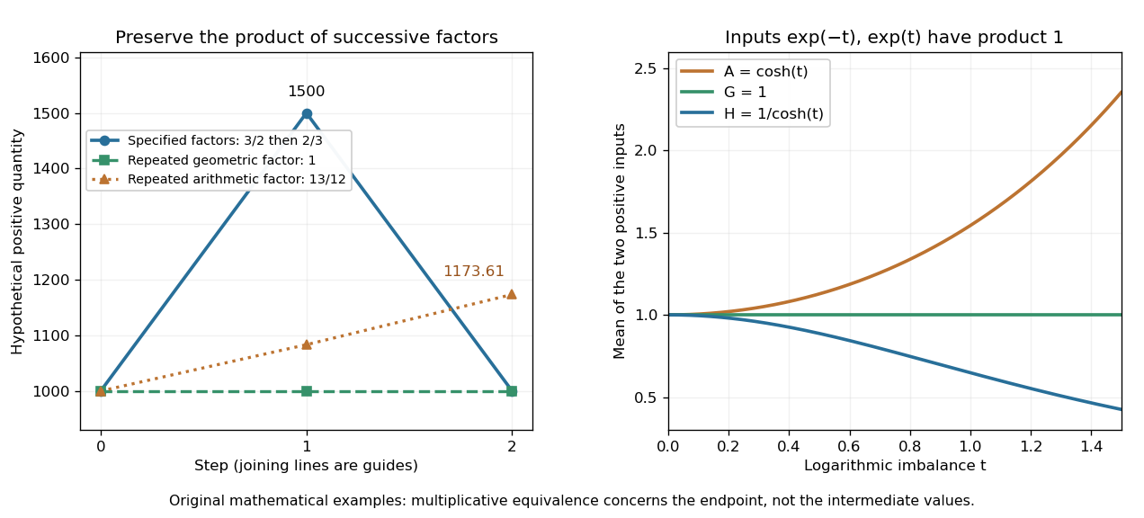
The geometric mean preserves multiplicative endpoints and sits between the harmonic mean and arithmetic mean
. Left: the original toy factors and return a quantity to its starting value; repeating their arithmetic mean would produce a larger endpoint. Right: the dimensionless inputs and keep product one while , , and separate as the inputs become less equal. Lines joining time steps are guides, not a continuous growth model. Details.The arithmetic-geometric mean inequality gives . Apply that same inequality to the multiplicative inverses to obtain , where is the harmonic mean. Consequentlyfor positive inputs, with equality throughout exactly when all inputs agree. For and , the three values are , , and . They preserve, respectively, the sum of inverses, the product, and the sum. No one of these summaries preserves all three for unequal inputs.
For a compact continuous module over the Iwasawa algebra of a Zp-extension, lifts of a basis of generate . Their generated image is compact. The quotient satisfies ; in every finite continuous quotient, acts nilpotently, since the group action is pro-. Thus all finite quotients of vanish, and compactness gives .
Informed consent is voluntary agreement after receiving and understanding relevant information about an intervention or participation in research. In a clinical trial, the participant is informed about the study procedures, potential benefits and risks, alternatives and the option to decline or withdraw. Consent precedes randomization.
Image segmentation divides an image signal domain into regions according to a chosen criterion, such as approximately constant or smoothly varying intensity. The Mumford–Shah segmentation model balances fidelity, within-region smoothness and image edge length. An intensity segmentation need not coincide with semantic object identities.
The diatomic molecule containing one ordinary hydrogen nucleus and one deuterium nucleus is an isotopic form of molecular hydrogen. It has a weak electric dipole and can supply low-temperature molecular line cooling in primordial gas when its abundance is sufficient.
A law or statistical object is scale invariant if its form is unchanged by rescaling lengths, with any specified scaling weight for the fields. A dimensionless field's three-dimensional nonzero-mode power spectrum obeys when its statistics have this scaling. The meaning of invariance must specify whether zero modes and regulators are being transformed.
A biological cell is a membrane-bounded basic unit of living organization. In a cell-level experiment it can be an experimental unit, provided that treatment assignment and relevant interactions are handled at that level.
The shared architecture of cellular life combines a selective cell membrane, internal cytoplasm, inherited information in DNA, and ribosomes that assemble proteins. Metabolism supplies transformations of matter and energy needed for maintenance and growth. These components form a coupled system: a boundary retains useful molecules, enzymes organize chemical reactions, and inherited information supports rebuilding the machinery. See Clark, Douglas and Choi, Biology 2e: prokaryotic cells.
A worked structural comparison: in a typical prokaryote, DNA occupies a region without a surrounding cell nucleus; in a typical nucleated eukaryote, much of the DNA lies inside a membrane-bounded cell nucleus. Both still have a cell membrane, cytoplasm and ribosomes. The extra boundary compartmentalizes processes; it does not create a different basic principle of living organization. See Clark, Douglas and Choi, Biology 2e: eukaryotic cells.
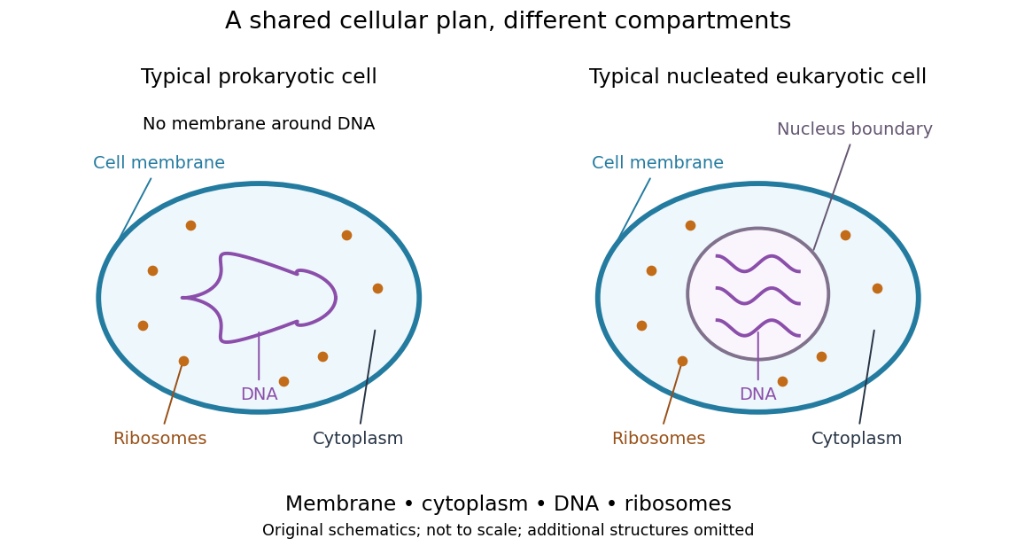
Shared cellular architecture with different DNA compartmentalization
. Original simplified schematics of a prokaryote and a nucleated eukaryote. Colors identify corresponding components; sizes and component counts are illustrative, and additional structures are omitted. Details.Shared architecture describes cellular life and its developmental machinery, rather than requiring every specialized biological cell to retain every component. A mature mammalian red blood cell, for example, lacks a cell nucleus, although it develops from nucleated precursors. See Clark, Douglas and Choi, Biology 2e: components of blood. This distinction makes cellular unity compatible with striking specialization.
For a potential already smooth on all of , the associated form is a Kähler form exactly when the displayed two positivity conditions hold. The first gives a positive metric coefficient off the origin; the second is positivity of . The associated real metric is . Positivity away from the origin alone permits a degenerate metric at the origin.
On a Riemann surface, the quotient sheaf records the finite negative Laurent series tails of meromorphic germs. At , a local coordinate identifies its stalk with . As a sheaf it is the direct sum of sheaves . Global sections prescribe locally finite families of principal parts, possibly infinite on a noncompact surface. The connecting homomorphism to is exactly the obstruction to a global meromorphic function with those parts and no extra poles.
The Kähler Laplacian identity implies that every holomorphic function on a Kähler manifold is a harmonic function. On functions, and by degree, so both terms of the Dolbeault Laplacian vanish. Compactness is unnecessary. Changing the sign convention for the scalar Laplacian does not change this conclusion.
For a tensor product of Lie algebra representations with weight-space decompositions, the weights add and their weight multiplicities convolve. A diagram must sum contributions landing at the same weight, rather than treating coincident points as distinct positions.
Pinned article: Introduction to the OurBigBook Project
Welcome to the OurBigBook Project! Our goal is to create the perfect publishing platform for STEM subjects, and get university-level students to write the best free STEM tutorials ever.
Everyone is welcome to create an account and play with the site: ourbigbook.com/go/register. We belive that students themselves can write amazing tutorials, but teachers are welcome too. You can write about anything you want, it doesn't have to be STEM or even educational. Silly test content is very welcome and you won't be penalized in any way. Just keep it legal!
Intro to OurBigBook
. Source. We have two killer features:
- topics: topics group articles by different users with the same title, e.g. here is the topic for the "Fundamental Theorem of Calculus" ourbigbook.com/go/topic/fundamental-theorem-of-calculusArticles of different users are sorted by upvote within each article page. This feature is a bit like:
- a Wikipedia where each user can have their own version of each article
- a Q&A website like Stack Overflow, where multiple people can give their views on a given topic, and the best ones are sorted by upvote. Except you don't need to wait for someone to ask first, and any topic goes, no matter how narrow or broad
This feature makes it possible for readers to find better explanations of any topic created by other writers. And it allows writers to create an explanation in a place that readers might actually find it.
Figure 1. Screenshot of the "Derivative" topic page. View it live at: ourbigbook.com/go/topic/derivativeVideo 2. OurBigBook Web topics demo. Source. - local editing: you can store all your personal knowledge base content locally in a plaintext markup format that can be edited locally and published either:This way you can be sure that even if OurBigBook.com were to go down one day (which we have no plans to do as it is quite cheap to host!), your content will still be perfectly readable as a static site.
- to OurBigBook.com to get awesome multi-user features like topics and likes
- as HTML files to a static website, which you can host yourself for free on many external providers like GitHub Pages, and remain in full control

Figure 2. You can publish local OurBigBook lightweight markup files to either OurBigBook.com or as a static website.
Figure 3. Visual Studio Code extension installation.
Figure 5. . You can also edit articles on the Web editor without installing anything locally. Video 3. Edit locally and publish demo. Source. This shows editing OurBigBook Markup and publishing it using the Visual Studio Code extension. 
- Infinitely deep tables of contents:




All our software is open source and hosted at: github.com/ourbigbook/ourbigbook
Further documentation can be found at: docs.ourbigbook.com
Feel free to reach our to us for any help or suggestions: docs.ourbigbook.com/#contact