A state $i$ is absorbing if $p_{ii}=1$, so once visited it is never left. Condition on the first step and use the Markov property: for $i\ne 1$, the subsequent probability of ever reaching state one is $h_j$ given $X_1=j$. Hence $h_i={\sum }_j{p}_{ij}{h}_j$, with $h_1=1$.

In this chain state four is a separate absorbing state, so $h_4=0$. The other two equations areSolving givesLet $t_i$ be the mean time to hit the absorbing set. From either transient state the next-step absorption probability is at least $1/3$, so its tail is geometrically bounded and the expectations are finite. First-step analysis gives $t_2=1+\frac{2}{3}{t}_3$ and $t_3=1+\frac{1}{4}{t}_2$. Thus $t_3=5/4+t_3/6$ and

The unit disk has area $\pi$, so its joint density is $f_{X,Y}(x,y)={\pi }^{-1}{1}_{\{x^2+y^2\le 1\}}$. The polar-coordinate Jacobian has absolute determinant $r$. Thereforeand is zero outside this rectangle, up to irrelevant boundary choices. Integrating givesThe joint density equals the product of the two marginal densities, so $R$ and $\Theta$ are independent. The angle at the centre can be chosen arbitrarily since that point has probability zero.

The Milne-Thomson circle theorem replaces a potential $f$ analytic inside the circle of radius $a$ by $f(z)+\overline{f(a^2/\bar{z})}$ outside it, when its original singularities are outside. The circle becomes a streamline, the imposed flow at infinity is preserved, and no extra circulation is introduced.

Use the convention that positive circulation is counterclockwise, so a vortex potential is $\Gamma \log (z-z_1)/(2\pi i)$ and its derivative is $u-iv$. With $b=a^2/{\bar{z}}_1$, the circle construction givesup to an additive constant and local logarithm branches. There is an image vortex of strength $-\Gamma$ at $b$ and a central vortex of strength $\Gamma$. Their zero net interior circulation is needed for the specified motion equation.

The original vortex moves with the regular velocity of the image flow, excluding its own singular velocity. ThusThe conjugation in this equation matches the printed source. Write $z_1=r{e}^{i\theta }$ and cancel $e^{-i\theta }$ to obtainReal and imaginary parts giveThe vortex moves uniformly on the circle determined by its initial radius, clockwise for positive $\Gamma$ in this convention.

Ampère's law in magnetostatics iswith boundary and surface orientations related by the right-hand rule. Stokes' theorem gives the left side as ${\int }_S(\nabla \times B)\cdot ndS$, proving the integral law from the stated curl equation.

For a circular contour of radius $r$ about the axis, the left side is $2\pi r{B}_{\theta }$. For $r\le a$ the enclosed current is $I{r}^2/a^2$; for $r\ge a$ it is $I$. ThereforeBoth expressions agree at the boundary. At the axis the field is zero, interpreted by continuity even though the angular unit vector is undefined there.

Time independence conserves the energy $E=T+mga\cos \theta$. The two cyclic coordinates giveThese are respectively angular momentum along the symmetry axis and angular momentum along the fixed upward vertical; $n$ is the axial spin rate. For $u=\cos \theta$ and $-1<u<1$, eliminate $\dot{\varphi }$ using $\dot{\varphi }=(h-Cnu)/[A(1-u^2)]$. The energy becomesMultiplying and rearranging givesTo justify the double-root condition, use the effective potentialEliminating the cyclic coordinates by Routh reduction gives the remaining equation $A\ddot{\theta }=-dU(\cos \theta )/d\theta$. A constant nonvertical angle therefore has $U^{\prime }(u_0)=0$ and $E=U(u_0)$. Since $P(u)=2A(E-U(u))(1-u^2)$, both $P(u_0)$ and $P^{\prime }(u_0)$ vanish. This argument uses the second-order equation; merely differentiating the energy identity at a stationary angle would not establish the derivative condition.

Thus steady nonvertical precession gives a common root in $(-1,1)$. The nonvertical qualification is implicit in the denominator used by the source. A top spinning exactly upright or inverted is also possible but corresponds to an endpoint $u=\pm 1$, not an interior root; the unrestricted literal claim would need that exception.

The distinction is captured by the double-root criterion for steady precession of a symmetric top.

Let $y_{ϵ}=y+ϵ\eta$, with $\eta ={\eta }^{\prime }=0$ at both endpoints. At an extremal the first variation is zero:Integrate the second term by parts once and the third term twice. The boundary term isThe given fundamental lemma therefore givesThis is the classical form under the usual smoothness hypotheses ensuring the displayed derivatives exist; without that extra regularity the variation first yields its distributional form.

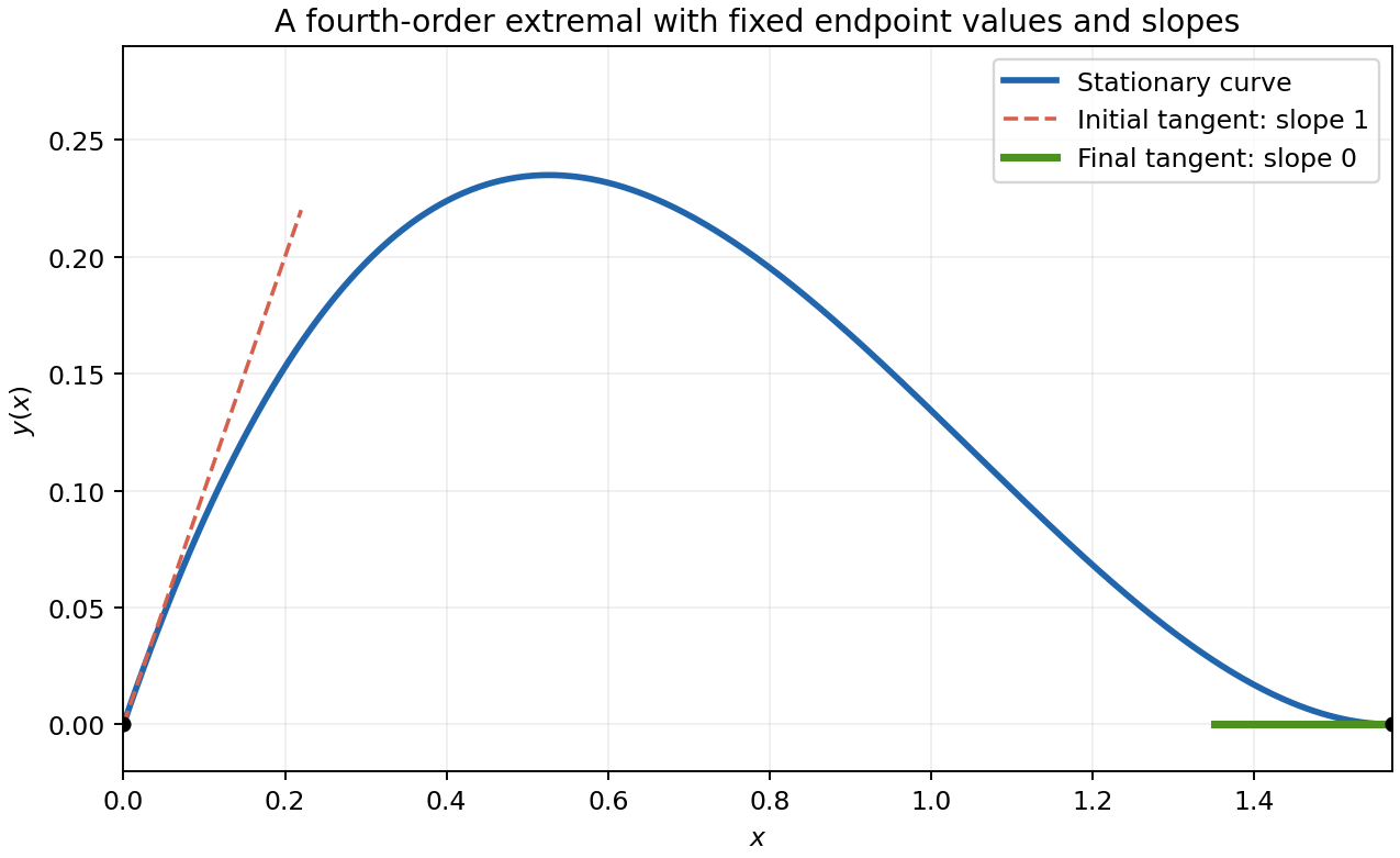
For the concrete functional the equation is $y^{(4)}-y=0$. Write $L=\pi /2$, $C=\cosh L$ and $S=\sinh L$. A general solution is $A\cos x+B\sin x+D\cosh x+E\sinh x$. The two initial conditions give $D=-A$ and $B+E=1$. The final derivative condition gives $A=EC/(1+S)$, and the final value condition then gives $E=(1+S)/2$. Thus an extremal isIt solves the differential equation, has initial value zero and initial derivative one, and at $L$ both its value and derivative vanish, using $C^2-S^2=1$. These checks verify all four prescribed endpoint conditions.

The implicit function theorem applies when $D_{2}F(a,b)\ne 0$. After shrinking the neighbourhood, this partial derivative stays nonzero along the implicit graph. Differentiating its defining identity givesFor the specified smooth function, $F_x=y+\cos (x+y)$ and $F_y=x+\cos (x+y)$, so both equal one at zero. In particular the theorem applies and $f^{\prime }(0)=-1$. Differentiate the identity a second time:At zero, $F_{xx}=F_{yy}=0$ and $F_{xy}=1$. Therefore

The subspace topology isThese sets contain the empty set and $A$, are closed under arbitrary unions, and are closed under finite intersections because intersections distribute over the common factor $A$. Thus they form a topology on $A$.

The sequence $x_n=1/(n+1)$ lies in the open interval and converges in the ambient real line to zero. Every subsequence also converges to zero, and uniqueness of limits prevents it converging to any point of the interval. Thus the interval is not sequentially compact.

For a sequence $(x_n,y_n)$ in the product, sequential compactness of $X$ supplies indices $n_j$ with $x_{n_j}\to x\in X$. Apply sequential compactness of $Y$ to the corresponding $y_{n_j}$, extracting a further subsequence $y_{n_{j_{\ell }}}\to y\in Y$. The first coordinate still tends to $x$. For any $ϵ>0$, both coordinate distances are eventually less than $ϵ/2$, so their sum is less than $ϵ$. Hence the same subsequence converges in the given product metric to $(x,y)$. This proves the product is sequentially compact.

A dominated differentiation theorem is the following. Suppose $\varphi (x,t)$ is measurable in $x$ and differentiable in $t$ on an open interval, is integrable for at least one parameter value, and its parameter derivative is dominated in absolute value by an integrable function independent of $t$. Then its integral is differentiable andLocal versions require the domination only on a neighbourhood of each parameter. The proof bounds the difference quotients by the dominating function, using the fundamental theorem of calculus or the mean-value theorem, then applies dominated convergence. Apply the argument to real and imaginary parts for a complex integrand.

For fixed $t$, $f(x)e^{itx}$ is measurable and has absolute value $|f(x)|$, so is integrable. Its derivative with respect to $t$ is $ixf(x)e^{itx}$, whose absolute value is the assumed integrable function $|xf(x)|$. HenceDominated convergence also shows this derivative is continuous, though only differentiability is required.