For the linear differential operator $L=D^2+4D+5$, the characteristic equation is $m^2+4m+5=0$, with roots $-2\pm i$. Take the fundamental system of solutionsThe Wronskian is never zero, so variation of parameters is valid on the whole interval. Write a particular solution as $a(x)u(x)+b(x)v(x)$, and impose the auxiliary condition $a^{\prime }u+b^{\prime }v=0$. Substitution then gives $a^{\prime }{u}^{\prime }+b^{\prime }{v}^{\prime }=f$. These two equations giveChoosing both integrals to start at zero makes the resulting particular solution and its first derivative vanish there:A general solution is $Au+Cv+y_p$. The boundary condition at zero sets $A=0$. The condition at $\ell =\pi /2$ givesbecause $\sin \ell =1$ and $\sin (\ell -t)=\cos t$. Combining the two integrals yields the Green's function representationIndeed, for $t<x$ the kernel is $-e^{2(t-x)}\sin t\cos x$, since $\sin (x-t)-\sin x\cos t=-\cos x\sin t$; for $x<t$ it is $-e^{2(t-x)}\sin x\cos t$.

For fixed interior $t$, the Green's function vanishes at both endpoints, is continuous at $x=t$, solves the homogeneous equation away from $t$, and satisfiesThis derivative jump is the normalization required by the leading coefficient one in $L$. Finally, a homogeneous solution satisfying the first boundary condition is $C{e}^{-2x}\sin x$, and the second boundary condition at $\pi /2$ forces $C=0$. Thus the boundary value problem has exactly one solution for every continuous forcing, justifying the unique inverse represented by this kernel.

The Bendixson-Dulac theorem states that if $(P,Q)$ is a continuously differentiable planar vector field on a simply connected open region $D$, and a continuously differentiable Dulac function $B$ makeshave one weak sign throughout $D$, without vanishing identically on any nonempty open subset, then there is no nonconstant periodic orbit contained in $D$. To see why, a hypothetical simple periodic orbit bounds a region in $D$. The divergence theorem gives the integral of this expression as the outward flux of $B(P,Q)$ across the orbit. The flux is zero because the vector field is tangent to its orbit, whereas the one-sign area integral is nonzero, a contradiction. The usual stricter version assumes a strictly positive or strictly negative expression everywhere.

For the printed polynomial system, the origin is an equilibrium andThus its linearization is a centre equilibrium. For the full system take $B=1$. The divergence isOn the open disk $x^2+y^2<3$ this is nonpositive, and is negative wherever $x\ne 0$. Its zero set inside the disk is a line, so it cannot vanish on any open subset. The Bendixson-Dulac theorem therefore provesThis also exposes a terminology problem in the source: a nonlinear centre equilibrium has surrounding closed orbits, so the printed claim of a centre cannot hold in that sense. The imaginary eigenvalues establish only a centre of the linearized system. In fact the full equilibrium is an asymptotically stable weak focus, as the following direct check shows.

A quartic Lyapunov correction for a weak focus makes the nonlinear damping visible. Put $r^2=x^2+y^2$ and consider the Lyapunov functionIt is positive definite sufficiently close to zero. Differentiating along the polynomial vector field givesFor clarity, the quartic terms come from $-x^4$ in the derivative of $r^2/2$, and from applying $y{\partial }_x-x{\partial }_y$ to the quartic correction. Their sum is $-3x^4/8-3x^2{y}^2/4-3y^4/8$; all other terms have degree at least six. Therefore $\dot{V}<0$ in a sufficiently small punctured neighbourhood, proving asymptotic stability by Second Lyapunov theorem. Finallyso nonconstant nearby orbits turn clockwise as they converge. The equilibrium is a weak focus despite the centre in its linearization. This interpretation resolves both the local dynamics and the absence of closed orbits without changing the printed coefficients.

The first component of the vector field vanishes only when $y=0$ or $x=\pm 1$. The second vanishes only when $y=1$ or $x+y=3$. Intersecting these alternatives gives exactly five equilibria. Their Jacobian matrix isAt $(3,0)$,The real parts are negative and the imaginary parts are nonzero, so $(3,0)$ is a stable spiral.

At $(1,1)$ the Jacobian matrix is $\mathrm{diag}(2,-1)$. Its real eigenvalues have opposite signs, so $(1,1)$ is a saddle equilibrium.

At $(1,2)$,Both eigenvalues are positive, so $(1,2)$ is an unstable node.

At $(-1,1)$ the Jacobian matrix is $\mathrm{diag}(-2,-3)$, giving a stable node.

At $(-1,4)$,so $(-1,4)$ is a saddle equilibrium. All five equilibria are hyperbolic, so these linear classifications determine their nonlinear local stability as well.

Use the branch of the complex logarithm with $0<\arg z<2\pi$, so the branch cut is the positive real axis, and take $\sqrt{z}=\exp (\mathrm{Log}z/2)$ on the same slit plane. Apply the residue theorem toon a positively oriented keyhole contour with inner radius $\rho <1$ and outer radius $R>1$. The upper bank travels from $\rho$ to $R$, the large circle counterclockwise, the lower bank from $R$ to $\rho$, and the small circle clockwise. One may first keep the banks at small nonzero angles and then take their limits.

On the upper bank, $\mathrm{Log}x=\log x$ and $\sqrt{x}$ is positive. On the lower bank, the corresponding limits are $\log x+2\pi i$ and $-\sqrt{x}$. Reversing the lower-bank orientation therefore makes the sum of the bank integrals tend toBoth are absolutely convergent: near zero compare with $x^{-1/2}(1+|\log x|)$, and near infinity with $x^{-5/2}(1+\log x)$. On the large circle, $|z^2+1|\ge R^2-1$, so its contribution is $O((\log R+1)R^{-3/2})$. On the small circle it is $O(\sqrt{\rho }(1+|\log \rho |))$. Both tend to zero.

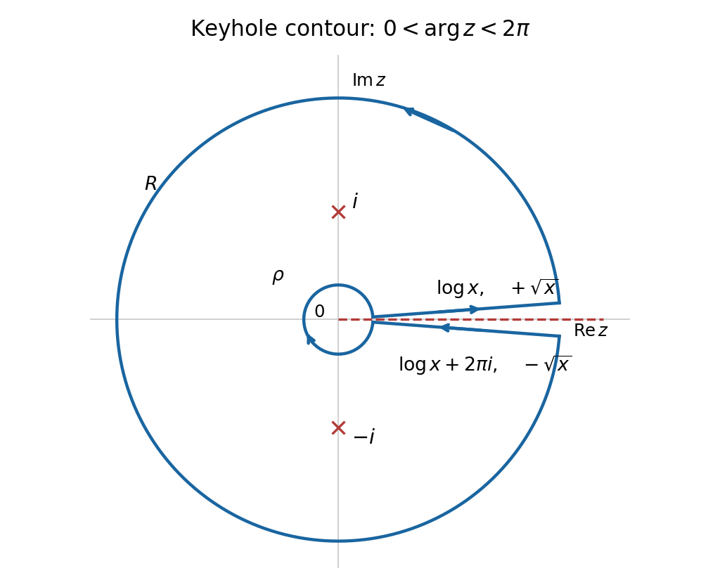
The two simple poles are $i$ and $-i$. On the chosen branch their arguments are $\pi /2$ and $3\pi /2$, respectively. Consequently their residues areFor example, the first follows from $\mathrm{Log}i=i\pi /2$, $\sqrt{i}=e^{i\pi /4}$ and the derivative $2i$ of the denominator factor $z^2+1$. The second uses $\sqrt{-i}=e^{3\pi i/4}$, rather than the value from the principal square-root branch. Adding and applying the residue theorem yieldsAs $J$ is real, taking real parts givesThe imaginary part also gives $J=\pi /\sqrt{2}$, an independent consistency check on the orientation and branch factors.

The tangent half-angle substitution $u=\tan (t/2)$ maps $0\le t<\pi$ to $0\le u<\infty$, withBecause $a>1$, both $a+1$ and $a-1$ are positive. ThusEvaluating the improper integral givesAlthough the change of variable has an infinite endpoint, the original integrand is continuous on the closed interval, and the transformed integrand decays as $u^{-2}$, so the limiting substitution is justified.

Inside the unit circle, use the geometric series for $1/(1-z)$:Outside the unit circle, expand in powers of $1/z$ instead:The different Laurent series reflect different annuli separated by the pole at one. Both follow from absolutely convergent geometric series in their stated regions.

The Laurent theorem states that a holomorphic function on the annulus $R<|z-a|<S$ has a unique Laurent seriesThe integration circle is counterclockwise. The series converges absolutely at every point of the annulus and uniformly on every compact subannulus. The coefficient integrals are independent of the choice of $\rho$ by the Cauchy integral theorem applied between two such circles. These statements include $R=0$ or $S=\infty$ when the indicated annulus has those endpoints.