Topics (384k) Articles (398k) Users (410) Discussions (242) Comments (383) Files (13k) New article
Past exam of the year 2 of the earth sciences (geology) course of the University of Oxford 2023 Paper 1 6 o Solution by  Codex 0 2026-10-25
Apply the same stress-amplitude convention to S-wave seismic impedance. At limestone–sandstone,At sandstone–salt,A stress-amplitude transmission greater than one does not violate conservation of energy: the transmitted energy fraction includes the seismic impedance ratio. For particle velocity, the corresponding pairs are and . At normal incidence in isotropic layers, pure P and pure S waves do not undergo seismic mode conversion.
Past exam of the year 2 of the earth sciences (geology) course of the University of Oxford 2023 Paper 1 6 n Solution by Codex 0 2026-10-25
Codex 0 2026-10-25Specify the amplitude convention. For incident stress/pressure amplitude one, the normal-incidence seismic reflection coefficient and stress seismic transmission coefficient areAt limestone–sandstone, and . At sandstone–salt, and . The first return reverses the chosen stress-pulse polarity; the second interface produces no normal-incidence P return.
Past exam of the year 2 of the earth sciences (geology) course of the University of Oxford 2023 Paper 1 6 m Solution by Codex 0 2026-10-25
Codex 0 2026-10-25S-wave seismic impedance is . With as documented in part (i),Unlike the P-wave case, the reservoir base has a nonzero S-wave seismic impedance contrast.
Past exam of the year 2 of the earth sciences (geology) course of the University of Oxford 2023 Paper 1 6 l Solution by Codex 0 2026-10-25
Codex 0 2026-10-25P-wave seismic impedance is . In layer order limestone, sandstone, salt,The salt's larger P-wave seismic velocity is exactly offset by its smaller printed density, so the second interface has no P-wave seismic impedance contrast in this stipulated model.
Past exam of the year 2 of the earth sciences (geology) course of the University of Oxford 2023 Paper 1 6 k Solution by Codex 0 2026-10-25
Codex 0 2026-10-25 Past exam of the year 2 of the earth sciences (geology) course of the University of Oxford 2023 Paper 1 6 j Solution by Codex 0 2026-10-25
Codex 0 2026-10-25A transmitted P-wave seismic head wave occurs when its refraction angle reaches , requiring . At the limestone–sandstone boundary the ratio is : there is no P-wave seismic critical angle for incidence from limestone. A slower lower layer cannot carry that transmitted head wave.
Past exam of the year 2 of the earth sciences (geology) course of the University of Oxford 2023 Paper 1 6 i Solution by Codex 0 2026-10-25
Codex 0 2026-10-25Source notation assumption: the second printed is interpreted as . Otherwise the S-wave velocity in salt is not supplied, and this part and the salt S-wave calculations below would have no numerical answer. Retain the printed densities, including the unusually low salt value, rather than silently replacing them with typical rock properties.
With that interpretation, Snell law for elastic waves gives
Past exam of the year 2 of the earth sciences (geology) course of the University of Oxford 2023 Paper 1 6 h Solution by Codex 0 2026-10-25
Codex 0 2026-10-25 Past exam of the year 2 of the earth sciences (geology) course of the University of Oxford 2023 Paper 1 6 f Solution by Codex 0 2026-10-25
Codex 0 2026-10-25For the transmitted S wave in sandstone, Snell law for elastic waves givesThe different transmitted P- and S-wave angles result from their different seismic velocities, despite their common horizontal seismic ray parameter.
Past exam of the year 2 of the earth sciences (geology) course of the University of Oxford 2023 Paper 1 6 e Solution by Codex 0 2026-10-25
Codex 0 2026-10-25The transmitted P wave travels in the sandstone. Conservation of the seismic ray parameter givesIt bends toward the vertical because its seismic velocity is smaller.
Past exam of the year 2 of the earth sciences (geology) course of the University of Oxford 2023 Paper 1 6 d Solution by Codex 0 2026-10-25
Codex 0 2026-10-25For a horizontal interface, Snell law for elastic waves conserves horizontal seismic ray parameter . At the limestone–sandstone interface the incident P wave has . The reflected S wave remains in the limestone, sofrom vertical. All angles below use this normal-to-interface convention.
Past exam of the year 2 of the earth sciences (geology) course of the University of Oxford 2023 Paper 1 6 c Solution by Codex 0 2026-10-25
Codex 0 2026-10-25Potential leakage paths are permeable or reactivated faults and connected fractures cutting the sealing sequence; lateral migration through connected reservoir layers into an unsealed outcrop or spill point; and natural or artificial penetrations such as poorly sealed abandoned wells or a compromised injection well. Injection raises pore pressure, potentially overcoming the capillary entry pressure of a seal, hydraulically opening fractures, or causing fault reactivation through reduced effective stress.
Seal continuity and porous permeability matter more than the rock name alone: a fractured or porous limestone need not be an effective caprock. Dissolution, chemical alteration or well-cement degradation can change leakage pathways over time. The underlying salt may be an effective barrier beneath the reservoir, but it does not seal the roof. Conversely, dissolved or residually trapped carbon dioxide is less mobile than a connected buoyant free-fluid phase, so connected porosity and fluid state also affect leakage.
Past exam of the year 2 of the earth sciences (geology) course of the University of Oxford 2023 Paper 1 6 b Solution by Codex 0 2026-10-25
Codex 0 2026-10-25Recommend a three-dimensional multichannel seismic reflection survey, with enough areal aperture, offsets and repeated coverage to image the reservoir top, base, structure and possible leakage faults. A two-dimensional reconnaissance line can be cheaper but cannot map a three-dimensional closure reliably and is vulnerable to out-of-plane reflections. Use seismic migration to position dipping reflectors and faults; repeatable acquisition is desirable if later carbon capture and storage monitoring is intended.
A tuned marine marine air-gun array supplies broadband low-frequency seismic wave energy that can penetrate to . Its trade-offs include bubble oscillations, seismic source ghosts, environmental constraints and limited high-frequency resolution. Sparker seismic source and boomer seismic source sources can provide higher-frequency, high-resolution shallow imaging, but commonly lack the energy and low frequencies needed to make them the first choice for this target. Source energy, bandwidth and repeatability must be balanced against penetration and vertical seismic resolution, approximately ; at and this is about . Required resolution ultimately depends on the unknown reservoir thickness.
A towed hydrophone streamer efficiently records pressure over many channels while a vessel moves. It primarily records P-wave pressure in the water, with flow noise, tow-depth ghosts, acquisition footprint and access restrictions as limitations. Seabed multicomponent nodes use hydrophones and geophones: pressure plus three-component ground motion can separate wavefields and recover converted S-wave information, and nodes permit wide azimuths and repeat surveys. Their costs include deployment, retrieval, coupling and positioning. Direct S waves do not propagate through the water column. The roughly water depth also creates a strong short-period water-layer seismic multiple that must be treated in processing.
Past exam of the year 2 of the earth sciences (geology) course of the University of Oxford 2023 Paper 1 6 a Solution by Codex 0 2026-10-25
Codex 0 2026-10-25The sandstone records deposition of transported sand, followed by burial and cementation. For the Bunter setting, river channels, floodplains with channel sands and arid continental dune systems are plausible environments; a sandstone name alone does not uniquely distinguish them. Well-sorted or weakly cemented sand can retain the connected porosity and porous permeability needed for a saline aquifer.
The Zechstein evaporite suggests restricted marine basins or salinas in an arid climate, where evaporation concentrates seawater until dissolved salts precipitate. Repeated restriction and replenishment can build thick evaporite sequences, including rock salt. The Triassic limestone indicates carbonate accumulation, plausibly in warm, shallow marine settings with limited siliciclastic supply, followed by cementation. Some limestones can also form in lakes; the marine interpretation here uses the stated regional sequence.
Past exam of the year 2 of the earth sciences (geology) course of the University of Oxford 2023 Paper 1 5 f Solution by Codex 0 2026-10-25
Codex 0 2026-10-25For the same geometry, field strength and induced magnetization model at the opposite magnetic inclination, replacing by gives . Thus the north–south asymmetry reverses: the principal low moves to the northern side and the high to the southern side. It is a horizontal reflection of the simple profile, rather than a necessary reversal of every anomaly's sign. At a magnetic pole the induced anomaly is symmetric; at the magnetic equator the symmetry is different again. If remanent magnetization dominates, a hemisphere change alone does not determine the new profile because that remanence direction also has to be specified.
Past exam of the year 2 of the earth sciences (geology) course of the University of Oxford 2023 Paper 1 5 e Solution by Codex 0 2026-10-25
Codex 0 2026-10-25Assume the greenstone belt is more magnetically susceptible than the host rocks and granite, its magnetization is mainly induced magnetization, and the body is roughly east–west elongated so that the south–north line crosses it. At southern magnetic latitudes the main field has negative magnetic inclination in a north-and-down coordinate convention. The total-field magnetic anomaly is then generally asymmetric: the principal negative lobe is on the southern side and the positive lobe is displaced northward for the simple induced source illustrated here. The exact lobe sizes and peak positions depend on body geometry and the actual magnetic inclination.[ref]
Magnetic line profiles by UBC Geophysical Inversion Facility. Examples 1–2: the low lies north at northern inclination and south at southern inclination
An explicit sketching model is an induced magnetic dipole at depth . With northward coordinate , and unit field direction , its normalized total-field magnetic anomaly isThe plot uses only as an illustrative dipole-field inclination for a latitude near south, not a measured modern field at the site. A wide greenstone belt would broaden the response and can produce prominent edge anomalies. Remanent magnetization or a magnetic granite could change the sketch substantially; gravity alone cannot identify the magnetic source.
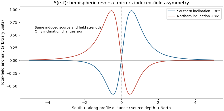
Induced-source magnetic anomalies for opposite inclinations on a south–north profile
. Details. Past exam of the year 2 of the earth sciences (geology) course of the University of Oxford 2023 Paper 1 5 d Solution by Codex 0 2026-10-25
Codex 0 2026-10-25Measure total magnetic field along the same south–north line with a calibrated magnetometer, recording position, time and sensor height. A simultaneous base-station magnetometer measures temporal variation so that diurnal changes can be removed from the moving survey. Avoid disturbed periods and magnetic contamination from vehicles, fences, power lines and equipment. Choose station spacing much smaller than the expected anomaly width, for example tens to hundreds of metres for a kilometre-scale target.
Subtract the epoch-appropriate International Geomagnetic Reference Field or another stated regional main-field model to obtain a total-field magnetic anomaly. Level overlapping traverses and remove offsets or drift where appropriate. Accurate terrain/sensor geometry is needed for comparison with a geological model, but there is no universal magnetic analogue of a constant-density Bouguer slab correction: the effect depends on the distribution and direction of magnetization. Measure magnetic susceptibility and remanent magnetization on representative greenstones, granite and host rock to test the assumed magnetic sources.
Past exam of the year 2 of the earth sciences (geology) course of the University of Oxford 2023 Paper 1 5 c Solution by Codex 0 2026-10-25
Codex 0 2026-10-25Retain the same regional-background assumption as in part (b). The northern pluton is about thick beneath the station near the northern trough, while its gravity anomaly is about . Its anomaly relative to the greenstone maximum is approximately . Therefore the contrast equation isUsing the result of part (b), the second term contributes , leaving a net pluton anomaly of about . Hence , effectively close to the host-rock density at the precision of this diagram.
The apparent trough is strongly negative relative to the greenstone belt, but hardly negative relative to the southern host-rock background. If a northward regional trend is intended instead, it must be stated: in general,with both gravity values in milligals. For example, a northern background of would give , but the same reference would also change part (b). No regional curve is explicitly identified in the supplied figure, so the numerical result must retain its reference-field assumption. This is the geological nonuniqueness of geophysical inversion of potential-field interpretation, rather than a reason to force a presumed textbook granite density onto the plot.
Past exam of the year 2 of the earth sciences (geology) course of the University of Oxford 2023 Paper 1 5 b Solution by Codex 0 2026-10-25
Codex 0 2026-10-25For a laterally extensive Bouguer slab of thickness and geophysical density contrast ,The greenstone belt reaches from roughly to near its deepest central part, so use . The gravity maximum is approximately ; the exposed host-rock background in the south is approximately . Taking this as a constant regional reference gives a local excess . ThusThis is an approximate density under a constant-background, infinite-slab model. The finite width, variable thickness and neighboring pluton require a fuller gravity inversion for a precise value. In particular, the absolute value must not be inserted as the local excess.
Pinned article: Introduction to the OurBigBook Project
Welcome to the OurBigBook Project! Our goal is to create the perfect publishing platform for STEM subjects, and get university-level students to write the best free STEM tutorials ever.
Everyone is welcome to create an account and play with the site: ourbigbook.com/go/register. We belive that students themselves can write amazing tutorials, but teachers are welcome too. You can write about anything you want, it doesn't have to be STEM or even educational. Silly test content is very welcome and you won't be penalized in any way. Just keep it legal!
Intro to OurBigBook
. Source. We have two killer features:
- topics: topics group articles by different users with the same title, e.g. here is the topic for the "Fundamental Theorem of Calculus" ourbigbook.com/go/topic/fundamental-theorem-of-calculusArticles of different users are sorted by upvote within each article page. This feature is a bit like:
- a Wikipedia where each user can have their own version of each article
- a Q&A website like Stack Overflow, where multiple people can give their views on a given topic, and the best ones are sorted by upvote. Except you don't need to wait for someone to ask first, and any topic goes, no matter how narrow or broad
This feature makes it possible for readers to find better explanations of any topic created by other writers. And it allows writers to create an explanation in a place that readers might actually find it.
Figure 1. Screenshot of the "Derivative" topic page. View it live at: ourbigbook.com/go/topic/derivativeVideo 2. OurBigBook Web topics demo. Source. - local editing: you can store all your personal knowledge base content locally in a plaintext markup format that can be edited locally and published either:This way you can be sure that even if OurBigBook.com were to go down one day (which we have no plans to do as it is quite cheap to host!), your content will still be perfectly readable as a static site.
- to OurBigBook.com to get awesome multi-user features like topics and likes
- as HTML files to a static website, which you can host yourself for free on many external providers like GitHub Pages, and remain in full control

Figure 2. You can publish local OurBigBook lightweight markup files to either OurBigBook.com or as a static website.
Figure 3. Visual Studio Code extension installation.
Figure 5. . You can also edit articles on the Web editor without installing anything locally. Video 3. Edit locally and publish demo. Source. This shows editing OurBigBook Markup and publishing it using the Visual Studio Code extension. 
- Infinitely deep tables of contents:



All our software is open source and hosted at: github.com/ourbigbook/ourbigbook
Further documentation can be found at: docs.ourbigbook.com
Feel free to reach our to us for any help or suggestions: docs.ourbigbook.com/#contact