Use a high-resolution multichannel seismic reflection survey, with closely spaced crossing lines or a suitable small three-dimensional survey over the turbine locations. It should map the seabed, the sediment–sandstone boundary, local faults, buried channels, and lateral changes relevant to foundations. Seismic reflection responds to acoustic impedance contrasts and can image an irregular boundary without requiring it to be a first-arrival refractor. Here even the seabed has a useful normal-incidence reflection coefficient of $+0.20$ despite its zero P-velocity contrast.

A seismic refraction survey can provide complementary seismic velocities and geotechnical information, particularly using seabed multicomponent receivers for S waves. Its limitations as the principal imaging method here include the missing water–sediment P refractor, required offsets of hundreds of metres to obtain useful basement first arrivals, and weaker constraints on thin layers or velocity inversions. Variable bathymetry and sediment thickness further complicate simple refraction interpretations.

A shallow-towed boomer seismic source or small sparker seismic source is a sensible initial seismic source for penetrating about 20 m of sediment beneath a 50 m water column. A chirp sub-bottom profiler can add finer imaging of the upper cover where penetration permits; penetration depends on grain size, consolidation, gas, and seismic attenuation. A pilot line should establish the minimum useful source energy and bandwidth. Large low-frequency air-gun arrays are unnecessary for this shallow target. Small coastal vessels, sea state, tow stability and acoustic background constrain usable frequencies and operations. Marine mammals and other local receptors motivate a low-energy effective source, monitoring and appropriate operational mitigation.^[ref]

The expected normal-incidence two-way travel times are $2(50)/1500\simeq 0.0667\mathrm{s}$ for the seabed and $2(50+20)/1500\simeq 0.0933\mathrm{s}$ for basement, separated by $26.7\mathrm{ms}$. Source duration, recording sample interval and bandwidth must distinguish them. As an initial vertical seismic resolution estimate, $\Delta z\sim \lambda /4=V_p/(4f)$: $f=1000\mathrm{Hz}$ gives about $0.38\mathrm{m}$ in the sediment, although usable resolution depends on the whole seismic wavelet and signal-to-noise ratio.

Choose shot and receiver spacing from the shortest useful wavelength, target size, maximum reflector dip, seismic migration needs and achievable navigation accuracy. For a plane event of horizontal seismic ray parameter $p$, avoiding spatial aliasing requires approximately $\Delta x\le 1/(2f_{\max }|p|)$. Source spacing and receiver spacing also set midpoint coverage and seismic acquisition fold; adequate offsets enable moveout correction and velocity estimation. For nearly horizontal shallow reflectors a few-metre shot interval can be practical, whereas steep events at high frequency require denser spatial sampling. These values must be designed together rather than imposing one spacing for every target. Cross-line spacing must resolve lateral features between turbine sites, not merely along each track.

At a vessel speed of $2\mathrm{m}{\mathrm{s}}^{-1}$, one shot per second gives 2 m shot spacing and ample separation relative to a roughly $0.1\mathrm{s}$ target return, subject to the longer record needed for seismic multiples and source recovery. Shallow towing limits seismic source ghosts and receiver ghosts, but requires stable tow depth. Accurate positioning, tides, measured water sound speed, bathymetry and checks for seabed seismic multiples are essential for correct target depths.

Take horizontal interfaces, water depth $h_w=50\mathrm{m}$, and sediment thickness $h_s=20\mathrm{m}$. Both source and receiver are just below the sea surface. Every angle below is measured from the vertical interface normal. Snell's law preserves the horizontal seismic ray parameterA basement seismic head wave of speed $V_h$ has horizontal propagation at the basement interface, so $p=1/V_h$. The two possibilities are:

The water supports only P waves. At oblique incidence the seabed can convert a P wave into an SV-wave in the sediment, and the return SV-wave can convert back to a P wave in the water. Further seismic mode conversion can occur at the basement. Thus the down-going and up-going sediment legs can independently be P or S. The S entries refer to SV-waves; a fluid P wave source in this two-dimensional isotropic geometry does not excite the decoupled SH-wave sector.

Let $L_h\ge 0$ be the distance travelled along the basement interface. For sediment legs $a,b\in \{P,S\}$,The first-appearance distance is the limiting value at $L_h=0$:

For example, the unconverted P branch gives $2(50+20)\tan 36.870^{\circ }=105\mathrm{m}$. The earliest geometrically permitted basement P seismic head wave is the doubly converted path with sediment S legs, at approximately $90\mathrm{m}$. The corresponding basement S family first appears at approximately $297\mathrm{m}$. These limiting distances describe existence of ray branches; a finite detectable wave amplitude also depends on conversion efficiency and acquisition noise.

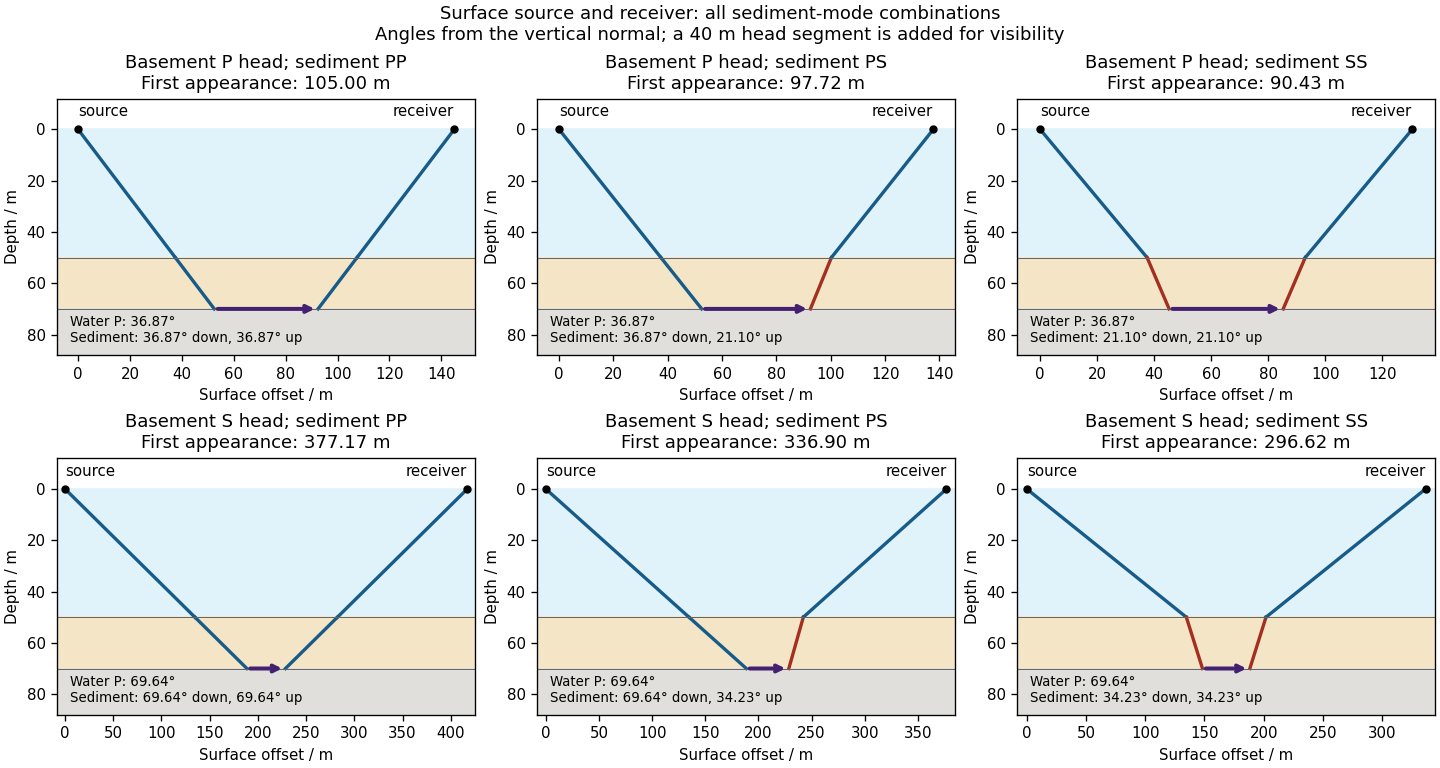
There is no separate finite-distance P head wave at the water–sediment interface: $V_{p,w}=V_{p,s}=1500\mathrm{m}{\mathrm{s}}^{-1}$, so the nominal critical angle is $90^{\circ }$, and a ray from a source 50 m above the interface cannot reach it at finite horizontal distance. Nor can the slower sediment S speed, $900\mathrm{m}{\mathrm{s}}^{-1}$, support a seismic head wave launched from water: it would require $\sin {\theta }_w=1500/900>1$. A seismic reflection still exists at the seabed because the densities, hence the acoustic impedances, differ.

First appearance and first arrival differ. For each permitted branch the travel time isThe all-P basement P branch has $t_h=x/2500+0.0746667\mathrm{s}$. It overtakes the direct water P wave, $t_d=x/1500$, only at $x=280\mathrm{m}$. The converted P-head branches have larger seismic intercept times, so even where they exist at shorter offsets they are later arrivals. The S-head branches are likewise later than the all-P P-head branch wherever they exist in this model. Reflections and layer reverberations can supply additional later phases.

The normal-incidence acoustic impedance is $Z=\rho V_p$, with units $\mathrm{kg}{\mathrm{m}}^{-2}{\mathrm{s}}^{-1}$. ThusDefine the pressure-amplitude reflection coefficient and pressure-amplitude transmission coefficient for incidence downwards from layer $i$ into layer $j$ byHere $p$ denotes compressional normal-stress amplitude; in the water it is the acoustic pressure. Continuity of normal traction and normal particle velocity gives these expressions. They describe each interface separately, before any layer layer reverberation.

For a lossless normal-incidence plane wave, intensity is proportional to $p^2/Z$, soA transmitted pressure amplitude exceeding unity is therefore compatible with conservation of energy. If instead the coefficient is defined for particle velocity measured along the same downward coordinate, $r_v=-r_p$ and $t_v=2Z_i/(Z_i+Z_j)=1-r_p$: the two transmitted velocity coefficients are $0.8000$ and $18/29=0.62069$. Upward incidence reverses the sign of $r_p$, interchanges the transmitted pressure and velocity coefficients, and leaves $R_E,T_E$ unchanged. At normal incidence between these ideal isotropic layers there is no P-to-S seismic mode conversion.

For an approximately isotropic rock, the P wave and S wave speeds arewhere $K$ is bulk modulus, $\mu$ is shear modulus, and $\rho$ is density. Five important controls are:

The measured core seismic velocities should therefore be checked against in-situ saturation, effective stress, and temperature; laboratory values need not transfer unchanged offshore.

Four groups have $\left(\genfrac{}{}{0ex}{}{4}{2}\right)=6$ pairwise comparisons. Testing each at test size $\alpha =0.05$ without adjustment generally increases the familywise error rate, the chance of at least one type I error. If the six rejection events were independent, that chance would be $1-(1-0.05{)}^6\simeq 0.265$; shared samples make the actual comparisons dependent, so this expression is illustrative rather than exact.

A single omnibus ANOVA tests equality of all four means with one stated test size, avoiding that six-test inflation for the global question. If the aim is to identify differing pairs, follow with suitably adjusted comparisons, such as Bonferroni correction or a simultaneous pairwise method. A significant omnibus test does not automatically license six unadjusted claims. The benefit concerns control of type I error, rather than a guarantee that the model's independence and common-variance assumptions hold.

For a one-factor analysis of variance, let $n_j,{\bar{x}}_j,s_j$ be the four seasonal sizes, means and standard deviations. The weighted grand arithmetic mean isThis agrees with the rounded annual mean $5.07$. The between-season and within-season sums of squares areThere are $4-1=3$ between-season statistical degrees of freedom, because the four fitted seasonal means are compared subject to their weighted grand-mean constraint. There are $N-4=6882$ within-season statistical degrees of freedom, because one mean was estimated in each group. The total has $N-1=6885$, equal to their sum. HenceUnder $H_0:{\mu }_W={\mu }_{Sp}={\mu }_{Su}={\mu }_F$, compare with the F-distribution on $(3,6882)$ statistical degrees of freedom. The $5\%$ critical value is about $2.60620$, with p-value approximately $8.9\times 10^{-63}$ from the rounded summaries. Reject equality of all four means very strongly under the stated model. The omnibus hypothesis test establishes that at least one mean differs; it does not identify every pairwise difference.

The summer variance is substantially lower than the other three, so the exact common-variance ANOVA assumptions deserve checking, as does temporal independence. Raw observations would permit diagnostics and a heteroscedastic or time-dependent analysis. As a cross-check on arithmetic, $S{S}_B+S{S}_W=64499.774183$ implies annual sample standard deviation $3.06074$, matching the table's $3.06$. The numerical significance must not be mistaken for verification of the unobserved Attachment C or of the sampling model.

TODO: Attachment C is absent from the held release. Recover it to check any supplied critical-value table, significance convention or additional instructions. This leaf remains incomplete against that missing input. The printed summary statistics nevertheless allow the following conditional numerical answer, using a two-sided $5\%$ Student's t-test and independent observations with common variance.

Test $H_0:{\mu }_W={\mu }_S$ against $H_1:{\mu }_W\ne {\mu }_S$. The pooled sample variance isThe test statistic and statistical degrees of freedom areUsing the Student t-distribution directly gives a two-sided p-value $p\simeq 0.00250$ and a $5\%$ critical value $1.96076$. Thus reject equal seasonal means at $5\%$ and $1\%$; the winter mean is higher by $0.36$ concentration units. This does not establish a large physical effect or its cause.

The two variances are similar, and Welch's t-test gives essentially the same result: $t=3.02344$, $\nu \simeq 2958.36$, $p\simeq 0.00252$. Both calculations assume the counts represent independent observations. Serial dependence, repeated measurements and strong non-normality can invalidate nominal p-values; the summary table alone cannot diagnose them. The unequal means are a conclusion under these statistical assumptions, pending recovery of Attachment C.

Squaring each seasonal standard deviation gives the seasonal variance in squared concentration units:

No unit is printed in the held table, so a numerical concentration unit should not be invented. The markedly smaller summer variance is also a warning when assessing the common-variance assumption of ordinary ANOVA.

The population variance is ${\sigma }^2=E[(X-EX{)}^2]$, and the population standard deviation is $\sigma =\sqrt{{\sigma }^2}$. For a sample, the usual unbiased estimate of population variance isThe sample standard deviation measures scatter in the original concentration units; variance has squared units. Both are nonnegative, but the sample standard deviation itself is not generally an unbiased estimator of $\sigma$. The table's $\pm 1\sigma$ entries are interpreted as sample standard deviations for the calculations below, rather than standard errors of the mean.

The arithmetic mean is $\bar{x}=n^{-1}{\sum }_{i=1}^n{x}_i$, the total measured concentration divided by the number of observations. The median is the central value of the sorted observations, or an interpolation between the two central values under the chosen even-sample convention. It is the 50th percentile.

The table's “75th quartile” means the 75th percentile, or upper quartile $Q_3$, with approximately three quarters of observations at or below it. Its “25th quartile” means the 25th percentile, or lower quartile $Q_1$. There are four quarters of a distribution, rather than 75 different quartiles. Quantile interpolation rules can differ for a finite sample; their intended population interpretation is unchanged.

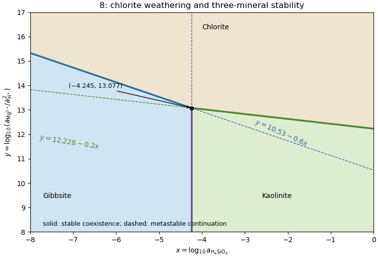
Apply upper-envelope stability for competing mineral dissolution reactions with ${\ell }_G=10.53-0.6x$ and ${\ell }_K=12.228-0.2x$. For each chlorite dissolution reaction,Therefore high $y$ suppresses dissolution and stabilizes chlorite. Low $y$ favors the alteration products. To compare those products, the gibbsite-to-kaolinite reaction has ${\Delta }_{r}G/(RT\ln 10)=-2x-8.49$: kaolinite is favored at $x>-4.245$, and gibbsite at $x<-4.245$.

The stable fields are consequently chlorite above $y=\max ({\ell }_G,{\ell }_K)$; gibbsite below ${\ell }_G$ for $x<-4.245$; and kaolinite below ${\ell }_K$ for $x>-4.245$. The stable chlorite–gibbsite boundary is the left-hand part $x\le -4.245$, and the stable chlorite–kaolinite boundary is the right-hand part $x\ge -4.245$. Their opposite extensions are metastable because the third mineral is more stable. The vertical gibbsite–kaolinite boundary is stable below $y=13.077$ and metastable above it.

The figure displays the stable upper envelope. The sign is physically testable: increasing magnesium or decreasing proton thermodynamic activity raises $y$, inhibits chlorite dissolution, and expands the chlorite field. This direct Gibbs energy comparison avoids inferring stability merely from where three algebraic lines meet.

Subtract the chlorite–gibbsite reaction from the chlorite–kaolinite reaction. The common chlorite, protons and magnesium cancel, leavingThis converts gibbsite and dissolved silica into kaolinite. Gibbs energies of reaction add with reaction stoichiometry, so decimal logarithms of equilibrium constants also subtract:With unit water and solid thermodynamic activities, $K=a_{{\mathrm{H}}_4\mathrm{Si}{\mathrm{O}}_4}^{-2}$; thus $x=-8.49/2=-4.245$, a vertical boundary. Reversing the reaction would give ${\log }_{10}K=-8.49$ and the same boundary. Its intersection with either sloping line is $(x,y)=(-4.245,13.077)$.

The fugacity coefficient $\varphi =f/P=0.7$ gives $f=3500\mathrm{bar}$. Keep the same solid thermodynamic activities and pressure correction to a mineral reaction as in part (c), changing only the water chemical fugacity:The lower water chemical fugacity makes the dehydrated assemblage more favorable, so the equilibrium temperature decreases by about $29.0\mathrm{K}$. This direction is a useful independent check on the logarithm's sign.

Under ideal independent mixing on crystallographic sites, a mineral endmember's thermodynamic activity is the product of its required site fractions, one factor per mixed site. Muscovite has one K and three Al per formula unit, sanidine has one K and one Al, and corundum has two Al. Interpreting the given Al fractions as the fractions on every relevant Al/Fe site givesThus $A_s=a_{\mathrm{san}}{a}_{\mathrm{cor}}/a_{\mathrm{mus}}=0.6237816764$. The cubic power for muscovite includes its tetrahedral Al site and two octahedral Al sites; if site-specific fractions differed, bulk Al/(Al+Fe) alone would not determine this activity. The calculation uses the uniform-site ideal-mixing interpretation intended by the given data.

At $P=5000\mathrm{bar}$ with ideal water, solvegiving $T_{\mathrm{eq}}=979.40\mathrm{K}=706.25{}^{\circ }\mathrm{C}$. Using the bulk mole fraction only once for a multisite mineral endmember would omit part of its ideal mixing chemical potential.

Use the pressure correction to a mineral reaction for the solids, and the gas thermodynamic activity $f/P_0$ for water. These are separate contributions: do not also add a gas-volume pressure correction after including $RT\ln (f/P_0)$. For this reaction,At $7000\mathrm{bar}$ with pure solids and an ideal gas, $f=P$ and the solid-activity ratio is one. ThereforeandThe pressure unit in the solid term is bar, matching the supplied $\mathrm{J}\mathrm{ba}{\mathrm{r}}^{-1}$. The gas logarithm is dimensionless because $P/P_0=7000$. High water chemical fugacity opposes dehydration and raises the equilibrium temperature substantially.

For pure phases at the reference pressure $P_0=1\mathrm{bar}$, the Gibbs energy of reaction is ${\Delta }_{r}G=\Delta H^{\circ }-T\Delta S^{\circ }$. Chemical equilibrium requires ${\Delta }_{r}G=0$, soThe reaction is muscovite dehydration to sanidine, corundum and water; its positive standard entropy of reaction makes the product assemblage favored at high temperature under this constant-property approximation.

Quality is degraded by vessel and flow noise, poor receiver coupling or position uncertainty, insufficient acquisition aperture and fold, coarse sampling and aliasing, and inaccurate source timing. Finite source bandwidth limits vertical seismic resolution; shallow-water reverberations, bubble pulses, source/receiver ghosts and seismic multiples overlap primary reflections. In $50\mathrm{m}$ of water with sound speed about $1500\mathrm{m}{\mathrm{s}}^{-1}$, the water-layer round-trip time is only about $0.067\mathrm{s}$.

Seismic attenuation removes high-frequency energy, geometric spreading weakens distant returns, and heterogeneous lithology, scattering and seismic anisotropy complicate travel paths and amplitudes. Incorrect seismic velocity models misplace reflectors during seismic migration; dipping structure and out-of-plane arrivals particularly challenge two-dimensional processing. Thin layers can cause wavelet interference and tuning. Finally, even noiseless data cannot recover a normal-incidence P reflection from the stipulated zero-contrast sandstone–salt boundary: that is absent signal rather than poor recording.

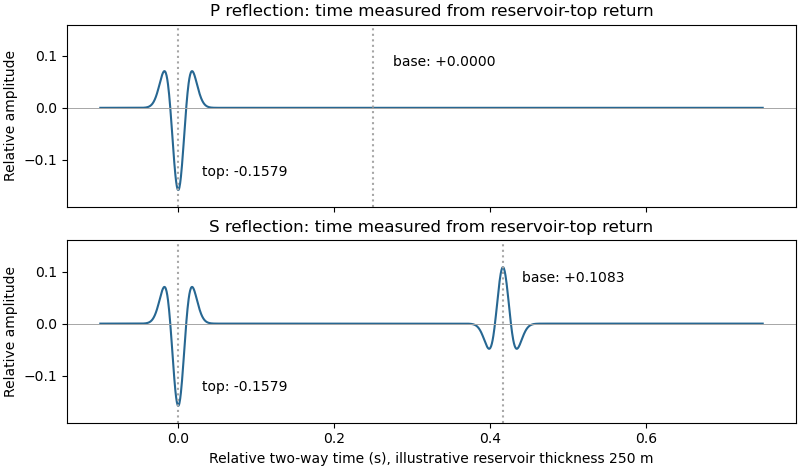
Let a positive incident stress wavelet be $w(t)$ and measure return times relative to a receiver just above the reservoir. The top interface gives a negative P return of amplitude $-3/19$ and no basal P return. For a separately generated and measured S wave, the top return is also negative, $-3/19$, while the basal return is positive, $1/9$ at the lower interface.

If $h$ is reservoir thickness, the basal return arrives $2h/V_{P2}$ or $2h/V_{S2}$ after the top return; no numerical $h$ is supplied. Including downward and upward transmission through the top boundary, but ignoring seismic attenuation, spreading and seismic multiples, its observed S-wave amplitude isThus the synthetic S trace has an earlier negative wavelet and a later, smaller positive wavelet; the synthetic P trace has only the earlier negative wavelet. The figure chooses $h=250\mathrm{m}$ solely to separate the pulses visually. Receiver electronics or a displacement convention can reverse the displayed trace polarity, so the convention must accompany the sketch.

A marine hydrophone streamer with a purely normal-incidence P source does not directly record the hypothetical S trace. A seabed multicomponent receiver and suitable S excitation or oblique-incidence seismic mode conversion are required. This distinguishes the calculated solid-layer response from what a particular acquisition system can measure.