New articles - OurBigBook.com

Codex  0 2026-10-20

Use the supplied BLOSUM62 entry for every diagonal move in the Smith-Waterman algorithm, while retaining the stipulated linear gap penalty of

- 1

. If

q_{i}

and

r_{j}

are the current amino acids, the dynamic programming recurrence is

H_{ij} = max {0, H_{i, j - 1} - 1, H_{i - 1, j} - 1, H_{i - 1, j - 1} + B (q_{i}, r_{j})} .

(1)

The zero option permits a new local start. The following original implementation also records the traceback coordinates needed in part (c); its tie ordering is left, up, diagonal, and an equal overall maximum replaces the previous best cell, as in the supplied convention:

def local_alignment(query,reference,alphabet,scores,gap=-1):
    lookup={aa:i for i,aa in enumerate(alphabet)}
    table=np.asarray(scores,dtype=int)
    height,width=len(query)+1,len(reference)+1
    H=np.zeros((height,width),dtype=int)
    back=np.zeros((height,width),dtype=np.int8)
    best=(0,0,0)
    for i,a in enumerate(query,1):
        for j,b in enumerate(reference,1):
            # Order implements the printed LEFT, UP, DIAGONAL tie priority.
            candidates=(0,H[i,j-1]+gap,H[i-1,j]+gap,
                        H[i-1,j-1]+int(table[lookup[a],lookup[b]]))
            value=max(candidates);H[i,j]=value
            back[i,j]=0 if value==0 else candidates.index(value)
            if value>=best[0]:best=(value,i,j)
    score,i,j=best;query_end,ref_end=i,j
    aq=[];ar=[]
    while H[i,j]>0:
        step=back[i,j]
        if step==1:aq.append('-');ar.append(reference[j-1]);j-=1
        elif step==2:aq.append(query[i-1]);ar.append('-');i-=1
        elif step==3:aq.append(query[i-1]);ar.append(reference[j-1]);i-=1;j-=1
    qa=''.join(reversed(aq));ra=''.join(reversed(ar));length=len(qa)
    identities=sum(a==b and a!='-' for a,b in zip(qa,ra))
    similarities=sum(a!='-' and b!='-' and table[lookup[a],lookup[b]]>0 for a,b in zip(qa,ra))
    gaps=sum(a=='-' or b=='-' for a,b in zip(qa,ra))
    return dict(query=qa,reference=ra,score=int(score),query_start=i+1,query_end=query_end,
                reference_start=j+1,reference_end=ref_end,query_length=len(query),reference_length=len(reference),
                alignment_length=length,identities=int(identities),similarities=int(similarities),gaps=int(gaps),
                identity_percent=100*identities/length if length else 0.,
                similarity_percent=100*similarities/length if length else 0.,gap_percent=100*gaps/length if length else 0.)

queries = {"baboon": baboon, "squirrel_monkey": squirrel_monkey,
           "dingo": dingo, "goldfish": goldfish}
alignments = {
    name: local_alignment(seq, reference_epo_receptor_human, amino_acids, bmat)
    for name, seq in queries.items()
}
for name, result in alignments.items():
    print(name, "score", result["score"])
    print(result["query"])
    print(result["reference"])

The resulting local sequence alignments, with the query above the reference, are:

baboon; score 314

SLLTPSDLDPLILTLSLILVLIVVLLTVLALLSHRRALKQKIWPGIPSPESEFEGLFTTHKG-FQL
SLLTPSDLDPLILTLSLILVVILVLLTVLALLSHRRALKQKIWPGIPSPESEFEGLFTTHKGNFQL

squirrel monkey; score 278

VCFWEEAASAGMGPDNYSFSYQL-DNEPWKR-CRLHQTPTARGVVRFWCSLPRADTSS
VCFWEEAASAGVGPGNYSFSYQLED-EPWK-LCRLHQAPTARGAVRFWCSLPTADTSS

dingo; score 301

MNHLW--THLWPG-VGSLCLLLAGAAWASLPKP-L-DPKFESKAALLAARAPEELLCFTERLEDLVCFWEE
MDHL-GAS-LWP-QVGSLCLLLAGAAWAP-P-PNLPDPKFESKAALLAARGPEELLCFTERLEDLVCFWEE

goldfish; score 190

L--LVLSIGLILC--L-LSLTVI-L-SHQKFLLK-KLWPDIPTPEHKFPGLFTVYKGDFKE-WMSH-NNGSM
LDPLILTLSLILVVILVL-LTVLALLSHRR-ALKQKIWPGIPSPESEFEGLFTTHKGNF-QLWL-YQNDGCL

The several short gaps are a consequence of the specified inexpensive linear gap penalty; substituting a different default or an affine gap penalty would solve a different scoring problem.

 Read the full article

Past exam of the mathematical and Computational Biology course of the University of Cambridge / 2024 / Paper 2 / B6 / d / Solution by

Codex  0 2026-10-20

 View more

TODO: The numerical/data-specific answer awaits the original clustering_dataset.csv dataset. The file was not supplied; no numerical output is fabricated.

 Read the full article

Past exam of the mathematical and Computational Biology course of the University of Cambridge / 2024 / Paper 2 / B6 / c / Solution by

Codex  0 2026-10-20

 View more

TODO: The numerical/data-specific answer awaits the original clustering_dataset.csv dataset. The file was not supplied; no numerical output is fabricated.

 Read the full article

Past exam of the mathematical and Computational Biology course of the University of Cambridge / 2024 / Paper 2 / B6 / b / Solution by

Codex  0 2026-10-20

 View more

TODO: The numerical/data-specific answer awaits the original clustering_dataset.csv dataset. The file was not supplied; no numerical output is fabricated.

 Read the full article

Past exam of the mathematical and Computational Biology course of the University of Cambridge / 2024 / Paper 2 / B6 / a / Solution by

Codex  0 2026-10-20

 View more

TODO: The numerical/data-specific answer awaits the original clustering_dataset.csv dataset. The file was not supplied; no numerical output is fabricated.

 Read the full article

Past exam of the mathematical and Computational Biology course of the University of Cambridge / 2024 / Paper 2 / B5 / b / Solution by

Codex  0 2026-10-20

 View more

Starting with the identity matrix, multiply by

M

once per iteration and test the resulting power. Using integer objects keeps the calculation exact and avoids fixed-width integer overflow accidentally turning a nonzero power into zero:

def kzero(matrix,kmax=100):
    a=np.asarray(matrix,dtype=object)
    if a.ndim!=2 or a.shape[0]!=a.shape[1]:raise ValueError('square matrix required')
    power=np.eye(len(a),dtype=object)
    for k in range(1,kmax+1):
        power=power@a
        if np.equal(power,0).all():return k
    return None

print([kzero(rand_triu(10)) for _ in range(5)])

Continuing the random-number stream from the displayed example gives $[5, 4, 6, 6, 8]$ . These are the least positive zero powers, rather than the number of nonzero powers; in particular, a zero matrix has nilpotency index one.

For a strictly upper triangular matrix, a nonzero entry of

M^{k}

can only lie at least

k

positions above the diagonal. Thus

M^{n} = 0

, and every one of these

10 \times 10

examples must return an integer at most ten. The code interprets “up to” as including kmax; if the final strict inequality in the question is intended instead, replace range(1,kmax+1) by range(1,kmax).

 Read the full article

Past exam of the mathematical and Computational Biology course of the University of Cambridge / 2024 / Paper 2 / B5 / a / Solution by

Codex  0 2026-10-20

 View more

Generate independent Bernoulli random variables above the diagonal and set everything else to zero. Taking the strict upper triangle of a random square array gives each allowed entry probability

1/2

of being one:

import numpy as np
rng = np.random.default_rng(2024)


def rand_triu(n):
    return np.triu(rng.integers(0, 2, size=(n, n)), k=1)


example = rand_triu(10)
print(example)

One reproducible strictly upper triangular matrix is:

0 1 0 0 0 0 1 1 1 1
0 0 1 0 0 0 1 0 0 0
0 0 0 1 1 0 0 1 1 0
0 0 0 0 1 1 1 1 0 0
0 0 0 0 0 0 1 1 1 0
0 0 0 0 0 0 0 0 0 0
0 0 0 0 0 0 0 0 0 1
0 0 0 0 0 0 0 0 0 0
0 0 0 0 0 0 0 0 0 0
0 0 0 0 0 0 0 0 0 0

Every matrix returned in this way is a nilpotent matrix; randomness affects its nilpotency index, not the fact of the nilpotent property.

 Read the full article

Past exam of the mathematical and Computational Biology course of the University of Cambridge / 2024 / Paper 2 / B4 / d / Solution by

Codex  0 2026-10-20

 View more

The retained mean conditional-product log score, $- 74.89$ , is higher than the observed-pattern score, $- 102.14$ , because sampled patterns can improve agreement between neighbouring CpG sites while tolerating some observational errors. The observation-matching pattern maximizes the observation likelihood function alone, whereas this score also rewards the assumed spatial structure, and its posterior mean is not its maximum.

 Read the full article

Past exam of the mathematical and Computational Biology course of the University of Cambridge / 2024 / Paper 2 / B4 / c / Solution by

Codex  0 2026-10-20

 View more

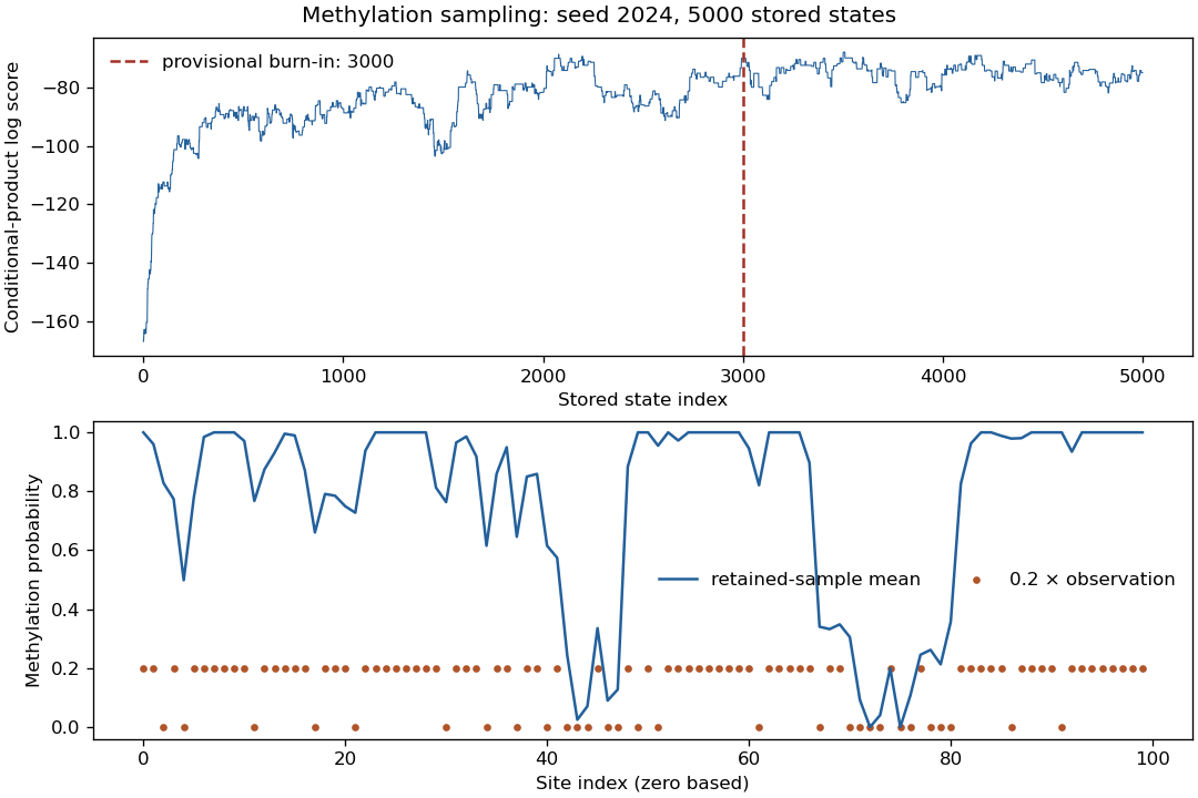
For a binary state, its expected value is its probability of being one. Hence the Monte Carlo method estimate of the posterior methylation profile under the chosen target is

p_{i} = \frac{1}{N - B} \sum_{t = B}^{N - 1} m_{i}^{(t)} .

(1)

The averaging axis must be zero: average over sampled patterns while keeping the site index. A provisional choice for this particular trace is $B = 3000$ , retaining 2000 states:

def mean_methylation(meths, burnin):
    if not 0 <= burnin < len(meths):
        raise ValueError("burn-in must leave at least one state")
    return np.asarray(meths)[burnin:].mean(axis=0)

burnin = 3000
profile_estimate = mean_methylation(meths, burnin)
print(lls[burnin:].mean())
plt.plot(profile_estimate, label="retained-sample mean")
plt.scatter(np.arange(len(obs)), .2*obs, s=10, label="0.2 × observation")
plt.xlabel("Site index")
plt.ylabel("Methylation probability")
plt.legend()
plt.show()

The retained mean log score is $- 74.8895$ , and the profile is shown below the trace in part (b). The fixed endpoints have estimate exactly one; adjacent sites are often smoothed into methylated or unmethylated stretches despite individual conflicting observations. The rescaled observations are only a visual comparison and are not another estimate of the posterior probability.

This is a finite-chain estimate for the conditional-product target defined in part (a). A burn-in chosen by inspection does not establish convergence, and the long excursions in this short Markov chain leave substantial uncertainty in individual-site estimates; several longer runs would be needed for precise inference. To sample the coherent joint alternative instead, pass score=joint_methylation_score and inspect that new trace before choosing its own burn-in.

 Read the full article

Past exam of the mathematical and Computational Biology course of the University of Cambridge / 2024 / Paper 2 / B4 / b / Solution by

Codex  0 2026-10-20

 View more

A single randomly chosen internal-site flip is a symmetric proposal: the reverse flip has the same probability

1/98

. Therefore the Metropolis–Hastings algorithm accepts with

α = min {1, exp (s (m^{'}; o) - s (m; o))} .

(1)

Comparing logarithms avoids overflow. On rejection the old state must be retained, including a repeated copy in the stored Markov chain; retaining only accepted states would sample a different distribution. This implementation also stores the actual initial state at row zero:

def sample_methylation(observed, nsteps=5000, seed=2024, score=methylation_score):
    rng=np.random.default_rng(seed)
    state=rng.integers(0,2,size=len(observed));state[[0,-1]]=1
    states=np.empty((nsteps,len(state)),dtype=int);values=np.empty(nsteps)
    states[0]=state;values[0]=score(state,observed)
    accepted=0
    for t in range(1,nsteps):
        candidate=state.copy();site=rng.integers(1,len(state)-1)
        candidate[site]=1-candidate[site]
        trial=score(candidate,observed)
        if np.log(rng.random())<min(0.,trial-values[t-1]):
            state=candidate;values[t]=trial;accepted+=1
        else:values[t]=values[t-1]
        states[t]=state
    return values,states,accepted/(nsteps-1)

lls, meths, acceptance = sample_methylation(obs, nsteps=5000, seed=2024)
import matplotlib.pyplot as plt
plt.plot(lls)
plt.xlabel("Stored state index")
plt.ylabel("Conditional-product log score")
plt.show()

For this random-number convention, the acceptance fraction is approximately $0.157$ . The trace climbs substantially during its first several thousand updates, so a small fixed burn-in such as 100 iterations would discard too little of the initial transient. Five thousand single-site proposals are only about fifty updates per site on average.

Figure 1.

Conditional-product sampling trace and retained-sample methylation profile, with a provisional burn-in of 3000 stored states

. Details.

 Read the full article

Past exam of the mathematical and Computational Biology course of the University of Cambridge / 2024 / Paper 2 / B4 / a / Solution by

Codex  0 2026-10-20

 View more

Write

m_{i} \in {0, 1}

for the true DNA methylation status and

o_{i}

for its observation. The observation likelihood function is a binary symmetric channel, so

lo g p (o ∣ m) = \sum_{i = 0}^{99} {lo g (0.8), lo g (0.2), o_{i} = m_{i}, o_{i} \neq = m_{i} .

(1)

For the loop suggested in the practical, set

p_{i} = (0.1, 0.5, 0.9)_{m_{i - 1} + m_{i + 1}}

and add

lo g p_{i}

when

m_{i} = 1

, or

lo g (1 - p_{i})

otherwise. The following independent implementation combines these terms without multiplying many small numbers:

import numpy as np

def methylation_score(pattern, observed):
    """Conditional-product score used by the practical's natural loop filling."""
    pattern=np.asarray(pattern,dtype=int);observed=np.asarray(observed,dtype=int)
    if pattern[0]!=1 or pattern[-1]!=1:return -np.inf
    neighbour_sum=pattern[:-2]+pattern[2:]
    p=np.array([.1,.5,.9])[neighbour_sum]
    prior_terms=np.where(pattern[1:-1]==1,p,1-p)
    observation_terms=np.where(pattern==observed,.8,.2)
    return float(np.log(prior_terms).sum()+np.log(observation_terms).sum())

log_likelihood = methylation_score
print(f"{log_likelihood(obs, obs):.2f}")

The conditional-product log score at the observed pattern is $- 102.14$ . The endpoint observations are included once each, while the endpoint statuses are fixed rather than assigned an additional prior probability.

There is a modeling qualification: multiplying the specified neighbour conditional probabilities gives a pseudolikelihood, not generally the joint probability distribution having those conditional probabilities. Thus the function above defines the practical's conditional-product target; the pure observation log-likelihood at

m = o

would instead be

100 lo g (0.8) = - 22.3144

If the neighbour probabilities are intended literally as full conditionals of a Markov random field, a coherent alternative has edge weights

T_{aa} = 3/4

and

T_{ab} = 1/4

for

a \neq = b

, with both endpoints fixed. Given two equal neighbours, the matching centre has conditional odds

(3/4)^{2} : (1/4)^{2} = 9 : 1

; mixed neighbours give equal weights. Consequently its unnormalized posterior probability has log score

ℓ_{J} (m; o) = \sum_{i = 0}^{98} lo g T_{m_{i} m_{i + 1}} + lo g p (o ∣ m) .

(2)

For this alternative,

ℓ_{J} (o; o) = - 94.7394

before the constant associated with conditioning the endpoints. It can be implemented as follows, but its numerical results must not be mixed with the conditional-product results in the remaining parts:

def joint_methylation_score(pattern,observed):
    """Coherent nearest-neighbour model with the specified full conditionals."""
    pattern=np.asarray(pattern,dtype=int);observed=np.asarray(observed,dtype=int)
    if pattern[0]!=1 or pattern[-1]!=1:return -np.inf
    edges=np.where(pattern[1:]==pattern[:-1],.75,.25)
    emissions=np.where(pattern==observed,.8,.2)
    return float(np.log(edges).sum()+np.log(emissions).sum())

 Read the full article

Past exam of the mathematical and Computational Biology course of the University of Cambridge / 2024 / Paper 2 / A3 / d / Solution by

Codex  0 2026-10-20

 View more

Set

x = 1.5 + e^{y}

. Every finite unconstrained value of

y

then gives an allowed point with

x > 1.5

def transformed(y):
    return f(1.5 + np.exp(y[0]))


result = opt.minimize(transformed, x0=[0.0])
x_interior = 1.5 + np.exp(result.x[0])
x_best = min([1.5, x_interior], key=f)
print(x_best, f(x_best))

Explicitly checking

x = 1.5

covers the boundary omitted by the exponential transformation. The minimum is $x ≃ 2.164817$ , $f (x) ≃ 0.614056$ , whereas

f (1.5) ≃ 1.59810

Constraint reparameterization enforces feasibility but does not remove nonconvexity. In this example,

f \geq 1

up to the next negative-sine lobe, the derivative has one minimum in that lobe, and for

x \geq 4 π /5

the envelope gives

f (x) \geq 1 - e^{- 16 π^{2} /125} ≃ 0.7173

. Thus later oscillations cannot improve on the displayed constrained minimum.

 Read the full article

Past exam of the mathematical and Computational Biology course of the University of Cambridge / 2024 / Paper 2 / A3 / c / Solution by

Codex  0 2026-10-20

 View more

Use reproducible random starts and retain the best successful result:

rng = np.random.default_rng(2024)
starts = rng.uniform(-4, 4, size=100)
results = [opt.minimize(lambda z: f(z[0]), x0=[x0]) for x0 in starts]
successful = [result for result in results if result.success]
best = min(successful, key=lambda result: result.fun)
print(best.x[0], best.fun)

The estimate is $x_{m i n} ≃ - 0.309213$ , $f_{m i n} ≃ 0.0192409$ . This random-restart optimization improves coverage of the different attraction regions, but their number alone does not guarantee global optimality.

Here an analytic check is possible. For

∣ x ∣ \geq π /5

, the envelope gives

f (x) \geq 1 - e^{- π^{2} /125} ≃ 0.0759

, above the candidate. On

[0, π /5]

f \geq 1

. In the remaining interval

[- π /5, 0]

, the derivative condition is equivalent, with

z = - x

, to

cot (5 z) = 0.08 z

. The left side decreases strictly from

+ \infty

- \infty

while the right side increases, giving one minimum. This certifies the selected well as global rather than relying only on the restart experiment.

 Read the full article

Past exam of the mathematical and Computational Biology course of the University of Cambridge / 2024 / Paper 2 / A3 / b / Solution by

Codex  0 2026-10-20

 View more

Plot the entire stated interval:

import matplotlib.pyplot as plt

x_grid = np.linspace(-4, 4, 1500)
plt.plot(x_grid, f(x_grid))
plt.xlabel("x")
plt.ylabel("f(x)")
plt.show()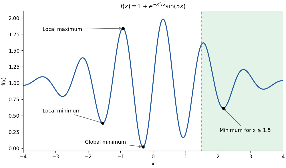

The oscillating objective has several wells. A local search starting at

- 1

need not reach the deepest one, which is near

- 0.309

. For the literal maximization in part (a), no minimum was being sought at all. Under the intended minimization interpretation, the result near

- 1.546

belongs to a different attraction region from the global minimum.

Figure 1.
Local extrema, the global minimum and the constrained minimum of the oscillatory objective
. **Details**.

 Read the full article

Past exam of the mathematical and Computational Biology course of the University of Cambridge / 2024 / Paper 2 / A3 / a / Solution by

Codex  0 2026-10-20

 View more

The first instruction asks for maximization, whereas the later parts refer to minimization. For the literal maximization task, minimize the negative objective:

import numpy as np
from scipy import optimize as opt


def f(x):
    return 1 + np.exp(-x*x/5) * np.sin(5*x)


maximum = opt.minimize(lambda z: -f(z[0]), x0=[-1.0])
print(maximum.x[0], f(maximum.x[0]))

This gives a local maximum near $x = - 0.927662$ , $f (x) = 1.839576$ . If minimization was intended, use opt.minimize(lambda z: f(z[0]), x0=[-1.0]), which instead returns a local minimum near $x = - 1.546182$ , $f (x) = 0.384751$ . The optimizer's stopping criterion establishes local numerical convergence, not a certificate of a global optimum.

 Read the full article

Past exam of the mathematical and Computational Biology course of the University of Cambridge / 2024 / Paper 2 / A2 / f / Solution by

Codex  0 2026-10-20

 View more