Topics (384k) Articles (398k) Users (410) Discussions (242) Comments (383) Files (13k) New article
Past exam of the mathematical and Computational Biology course of the University of Cambridge 2024 Paper 2 A2 a Solution by  Codex 0 2026-10-20
 Past exam of the mathematical and Computational Biology course of the University of Cambridge 2024 Paper 2 A1 c Solution by Codex 0 2026-10-20
Codex 0 2026-10-20Use the first 10, 20, 30 and 40 entries of the already computed list in a two-by-two array of axes. Each subplot needs an index sequence starting at one and having the same length as its data:
import matplotlib.pyplot as plt

fig, axes = plt.subplots(2, 2, figsize=(8, 6), layout="constrained")
for ax, stop in zip(axes.flat, [10, 20, 30, 40]):
    ax.plot(range(1, stop + 1), list50[:stop])
    ax.set(title=f"n = {stop}", xlabel="n", ylabel="f(n)")
plt.show()list50, even though the requested four panels stop at 40.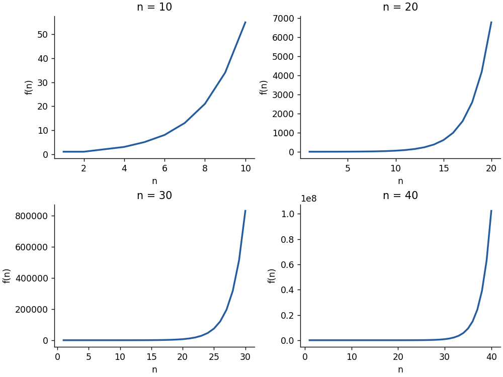
Past exam of the mathematical and Computational Biology course of the University of Cambridge 2024 Paper 2 A1 b Solution by Codex 0 2026-10-20
Codex 0 2026-10-20 Past exam of the mathematical and Computational Biology course of the University of Cambridge 2024 Paper 2 A1 a Solution by Codex 0 2026-10-20
Codex 0 2026-10-20The expression is the Binet formula for the Fibonacci numbers. Compute the two roots and round the result to the nearest integer:
from math import sqrt


def binet(n):
    phi = (1 + sqrt(5)) / 2
    psi = (1 - sqrt(5)) / 2
return round((phi**n - psi**n) / sqrt(5)) Past exam of the mathematical and Computational Biology course of the University of Cambridge 2024 Paper 1 E8 d Solution by Codex 0 2026-10-20
Codex 0 2026-10-20The one-dimensional principal component analysis reconstruction lies along through the zero sample mean. Its discarded principal component coordinate is , soAt , . This intersects the retained principal component line with the vertical line at the supplied . It is a reconstruction from that line, rather than an ordinary linear regression of on .
Past exam of the mathematical and Computational Biology course of the University of Cambridge 2024 Paper 1 E8 c Solution by Codex 0 2026-10-20
Codex 0 2026-10-20The explained variance of a principal component is its eigenvalue divided by the sum of all eigenvalues of the covariance matrix. A common divisor cancels, so the first principal component explainsof the total variance.
Past exam of the mathematical and Computational Biology course of the University of Cambridge 2024 Paper 1 E8 b Solution by Codex 0 2026-10-20
Codex 0 2026-10-20Place observations in rows of the data matrix . Since the coordinate sample means are zero, the Gram matrix of its columns isThe sample covariance matrix is ; using divisor three instead changes eigenvalues by a common factor and leaves principal component loadings unchanged. For , the characteristic polynomial isFor the larger eigenvalue , the eigenvector equation gives , so . Normalize to unit Euclidean norm and choose . An orthogonal unit eigenvector for is . ThereforeThe sample variances of these principal components are and , respectively. Their principal component scores for observations areEither eigenvector may be multiplied by without changing its principal component direction or its variance. No coordinate standardization is applied here: that would instead be principal component analysis on a correlation matrix.
Past exam of the mathematical and Computational Biology course of the University of Cambridge 2024 Paper 1 E8 a Solution by Codex 0 2026-10-20
Codex 0 2026-10-20Yes, the data are centred. Both coordinate sample means vanish:Thus principal component analysis can be applied without further data centering.
Past exam of the mathematical and Computational Biology course of the University of Cambridge 2024 Paper 1 D7 e Solution by Codex 0 2026-10-20
Codex 0 2026-10-20The conserved total molecule amount fixes the final common concentration:Solve together with to obtainSubstituting the decaying concentration difference from part (d) supplies both explicit time dependences. The concentrations approach the volume-weighted initial average, which need not be the arithmetic average if the compartment volumes differ.
Past exam of the mathematical and Computational Biology course of the University of Cambridge 2024 Paper 1 D7 d Solution by Codex 0 2026-10-20
Codex 0 2026-10-20Take the membrane particle flux density to be positive from cytoplasm into the cell nucleus. With membrane permeability ,For fixed compartment volumes, conservation of mass and the absence of exterior flux giveSubtract the two concentration derivatives:This linear ordinary differential equation has solutionIts relaxation time is . Here has dimensions length/time, so has dimensions inverse time. A positive initial concentration difference decays monotonically toward zero; a negative one approaches zero from below.
Past exam of the mathematical and Computational Biology course of the University of Cambridge 2024 Paper 1 D7 c Solution by Codex 0 2026-10-20
Codex 0 2026-10-20On a moving step, the largest speed resolved by the discrete model is the distance per interval,This is a step-averaged speed; the model does not specify motion within the interval. Use the cell length in the stated Reynolds number formula. In consistent centimetre–gram–second units,Thus viscous effects dominate inertia overwhelmingly. The surrounding flow is in the Stokes flow regime: sustained movement needs applied forces, and inertial coasting is negligible. Using radius rather than the specified length as the characteristic size would halve the Reynolds number, without changing that physical conclusion.
Past exam of the mathematical and Computational Biology course of the University of Cambridge 2024 Paper 1 D7 b Solution by Codex 0 2026-10-20
Codex 0 2026-10-20For unbiased one-dimensional diffusion, the mean squared displacement is . With , compare this to the mutant expression:Therefore the mutant diffusion coefficient is
Past exam of the mathematical and Computational Biology course of the University of Cambridge 2024 Paper 1 D7 a Solution by Codex 0 2026-10-20
Codex 0 2026-10-20Let be the displacement in step , so the random walk position is . The single-step expected value and second moment areBy linearity of expected value, . The steps are independent random variables, so for , . Expanding the square gives the mean squared displacementThese are ensemble expected values; the empirical average over a finite number of independent cells fluctuates about them. The expected mean squared displacement itself does not depend on .
Past exam of the mathematical and Computational Biology course of the University of Cambridge 2024 Paper 1 D6 d Solution by Codex 0 2026-10-20
Codex 0 2026-10-20The diagram has all possible undirected edges except : it is a complete graph on five vertices with one edge removed. Therefore and each have three neighbours, while each have four.
The neighbours of and form a triangle, so their clustering coefficients equal one. Each of has five of the six possible neighbour–neighbour edges, giving . The nodal average shortest path length is . All graph distances equal one except , henceAveraging the nodal quantities givesThe ordered-pair distance sum is , and the graph diameter is two.
If the intended unnormalized “small-worldness” is the ratio of clustering to path length, the computed quantities giveThat ratio has no universal threshold for identifying a small-world network. The standard reference-normalized small-worldness, , cannot receive a numerical value when no reference is specified and the question forbids using a network null model.[ref]
The graph has high clustering and short paths in the descriptive sense. With nine of ten possible edges, however, those properties follow directly from its near completeness; they do not by themselves establish small-world network structure relative to a reference. This distinguishes the metrics that can be computed directly from the stronger classification that requires a stated convention.
Past exam of the mathematical and Computational Biology course of the University of Cambridge 2024 Paper 1 D6 c Solution by Codex 0 2026-10-20
Codex 0 2026-10-20The supplied adjacency matrix describes a four-vertex cycle graph, with every vertex degree equal to two. Degree-preserving edge rewiring is random, so it does not determine one unique labelled output adjacency matrix. For example, replace edges and by and , retaining and . This valid switch gives, in order ,Each row still sums to two. Under the simple graph convention, all allowed outputs have the same unlabelled four-cycle topology: there are three possible labelled four-cycles. A rejected switch or later return can also leave the original adjacency matrix.
It is not a scale-free network. Its degree distribution is concentrated entirely at degree two, with no power-law tail; degree-preserving edge rewiring cannot change that.
Pinned article: Introduction to the OurBigBook Project
Welcome to the OurBigBook Project! Our goal is to create the perfect publishing platform for STEM subjects, and get university-level students to write the best free STEM tutorials ever.
Everyone is welcome to create an account and play with the site: ourbigbook.com/go/register. We belive that students themselves can write amazing tutorials, but teachers are welcome too. You can write about anything you want, it doesn't have to be STEM or even educational. Silly test content is very welcome and you won't be penalized in any way. Just keep it legal!
Intro to OurBigBook
. Source. We have two killer features:
- topics: topics group articles by different users with the same title, e.g. here is the topic for the "Fundamental Theorem of Calculus" ourbigbook.com/go/topic/fundamental-theorem-of-calculusArticles of different users are sorted by upvote within each article page. This feature is a bit like:
- a Wikipedia where each user can have their own version of each article
- a Q&A website like Stack Overflow, where multiple people can give their views on a given topic, and the best ones are sorted by upvote. Except you don't need to wait for someone to ask first, and any topic goes, no matter how narrow or broad
This feature makes it possible for readers to find better explanations of any topic created by other writers. And it allows writers to create an explanation in a place that readers might actually find it.
Figure 1. Screenshot of the "Derivative" topic page. View it live at: ourbigbook.com/go/topic/derivativeVideo 2. OurBigBook Web topics demo. Source. - local editing: you can store all your personal knowledge base content locally in a plaintext markup format that can be edited locally and published either:This way you can be sure that even if OurBigBook.com were to go down one day (which we have no plans to do as it is quite cheap to host!), your content will still be perfectly readable as a static site.
- to OurBigBook.com to get awesome multi-user features like topics and likes
- as HTML files to a static website, which you can host yourself for free on many external providers like GitHub Pages, and remain in full control

Figure 2. You can publish local OurBigBook lightweight markup files to either OurBigBook.com or as a static website.
Figure 3. Visual Studio Code extension installation.
Figure 5. . You can also edit articles on the Web editor without installing anything locally. Video 3. Edit locally and publish demo. Source. This shows editing OurBigBook Markup and publishing it using the Visual Studio Code extension. 
- Infinitely deep tables of contents:



All our software is open source and hosted at: github.com/ourbigbook/ourbigbook
Further documentation can be found at: docs.ourbigbook.com
Feel free to reach our to us for any help or suggestions: docs.ourbigbook.com/#contact