First perform the inner integral, which gives the vertical width of the region:Using $\int \sqrt{1-x^2}dx=\frac{1}{2}[x\sqrt{1-x^2}+\arcsin x]$ givesAt the intersection, $\sqrt{1-a^2}=a^2$, so

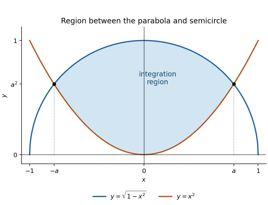
The region lies above the parabola $y=x^2$ and below the upper semicircle $y=\sqrt{1-x^2}$. Their intersections satisfy $x^4+x^2-1=0$, hence $x=\pm a$ with $a^2=(\sqrt{5}-1)/2$. In particular, $\sqrt{1-a^2}=a^2$. The region isIt is symmetric about the $y$ axis, with endpoints $(\pm a,a^2)$; at $x=0$ it extends from $y=0$ to $y=1$.

Height above the surface is $h=r-R$. Integrate the density over all exterior spherical shells:Repeated integration by parts, or the substitution $h=h_{0}s$, givesExpand $(R+h{)}^2$ and use these moments to obtain the mass of an exponential spherical atmosphere:For $h_0\ll R$, the leading term is surface area $4\pi R^2$ times column mass ${\rho }_0{h}_0$; the other terms retain the finite-curvature corrections.

In spherical coordinates, $\theta$ is the polar angle from the positive $z$ axis and $\varphi$ the azimuthal angle. The Jacobian determinant of the coordinate transformation gives the volume element

The function $g(x)=1/(x{\ln }^{2}x)$ is likewise positive and decreasing on $[2,\infty )$, with $g^{\prime }(x)=-(\ln x+2)/(x^2{\ln }^{3}x)<0$. NowThe integral test for convergence shows that $\sum _{n=2}^{\infty }1/(n{\ln }^{2}n)$ converges. This comparison integral determines convergence, not the numerical value of the series itself.

The function $g(x)=1/(x\ln x)$ is positive and decreasing for $x\ge 2$, since $g^{\prime }(x)=-(\ln x+1)/(x^2{\ln }^{2}x)<0$. The integral test for convergence therefore applies. Its comparison improper integral isConsequently $\sum _{n=2}^{\infty }1/(n\ln n)$ diverges.

Separate one factor of the hyperbolic sine and use the hyperbolic Pythagorean identity ${\sinh }^{2}x={\cosh }^{2}x-1$. With $u=\cosh x$ and $du=\sinh xdx$, integration by substitution givesFor real $x$, the hyperbolic cosine never vanishes. Differentiating the result gives $\sinh x(1-{\mathrm{sech}}^{2}x)={\sinh }^{3}x/{\cosh }^{2}x$, checking the sign of the reciprocal term.

Use integration by substitution with $u=\ln x$, so $du=dx/x$. For $x>1$, also $u>0$, andThe domain condition explains why no absolute value is needed around the inner logarithm.

The same integration by substitution gives the expected valueThe remaining integrand is an odd function. Its integral is absolutely convergent, since ${\mathrm{sech}}^{2}t\le 4e^{-2|t|}$ and $|t|e^{-2|t|}$ is integrable. Thus cancellation under symmetry in integration is legitimate, rather than merely a principal-value calculation. ConsequentlyEquivalently, the logistic distribution is symmetric about $\mu$, and its exponentially decaying tails ensure that its expected value exists.

For $s>0$, integrate the probability density function to obtain the cumulative distribution functionIf $\mu >0$, the requested probability is $F_X(\mu )-F_X(0)$. Since the hyperbolic tangent is odd, this givesThe second case matters because the question places no sign restriction on $\mu$: the event is empty when its upper endpoint is nonpositive. Using an oriented integral from $0$ to a negative $\mu$ would give a negative number, not a probability.

A probability density function must be nonnegative. The printed condition $s\ne 0$ is therefore too weak: for $s<0$ the given prefactor makes the function negative everywhere. The location-scale form of the logistic distribution requires $s>0$, which is assumed in the remaining parts.

Set $t=(x-\mu )/(2s)$, so $dx=2sdt$. The normalization of a probability distribution follows from the antiderivative of the squared hyperbolic secant:For completeness, the same expression with $s<0$ integrates to $-1$, since the transformed limits reverse. If a signed scale were desired, replacing its prefactor by $1/(4|s|)$ would give a valid density, but that is a correction to the printed formula.

The Maclaurin series give $e^{-x^3}=1-x^3+O(x^6)$ and $\cosh x=1+x^2/2+x^4/24+O(x^6)$. Inverting the latter using the geometric series givesMultiplying the two expansions yieldsThe remainder is $O(x^5)$ because the product already generates an $x^5$ term from $(-x^3)(-x^2/2)$.

Use the Maclaurin series $\sin x=x-x^3/6+O(x^5)$ and $e^u=1+u+u^2/2+u^3/6+u^4/24+O(u^5)$. The terms through fourth degree giveIn particular the cubic coefficient cancels; it has not been omitted accidentally.

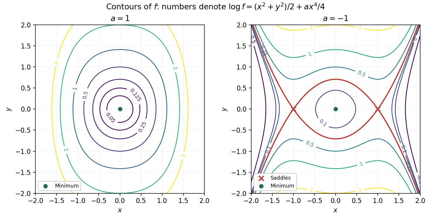
For $a=-1$, the local minimum at the origin has $f=1$. Its full level set isThe connected component containing the minimum is just the isolated origin. The same level also has the outer branches $y=\pm \sqrt{x^4/2-x^2}$ for $|x|\ge \sqrt{2}$; these are different connected components, not curves approaching the origin.

Both saddle points $(\pm 1,0)$ have $f=e^{1/4}$. Their common level set factors asIts explicit equations are thereforeThe two parabolas cross at each saddle, explaining the change of contour connectivity there. Each displayed equation can be restricted to the square of part (ii) if only that sketch window is wanted.

Because the exponential function is strictly increasing, the level sets $f=L>0$ are exactly those of $G=\ln L$. For $a=1$ they satisfyThere are no contours for $L<1$, the level $L=1$ is the origin, and $L>1$ gives nested closed ovals symmetric about both axes. Their stronger fourth-power growth in $x$ makes them relatively narrower horizontally as the level rises.

For $a=-1$, the contour equation becomesThe central local minimum is surrounded by closed ovals for $1<L<e^{1/4}$, accompanied by outer open branches. At $L=e^{1/4}$, the level passes through the two saddle points $(\pm 1,0)$ and changes its connectivity. Levels $L<1$ have only outer branches, while levels above the saddle value have an upper and a lower branch. The sketch is restricted to the requested square; labels give $G=\ln f$, so they identify the corresponding contours of $f$ without exponentially large labels.

Put $G=(x^2+y^2)/2+a{x}^4/4$, so $f=e^G>0$. Since $f_x=f{G}_x$ and $f_y=f{G}_y$, its stationary points satisfyThe origin occurs for every real $a$. There are two additional points only for $a<0$, at $x=\pm 1/\sqrt{-a}$.

At a stationary point, the Hessian matrix simplifies because $\nabla G=0$:At the origin this is $I$, so $(0,0)$ is a strict local minimum for every $a$, with $f=1$. If $a\ge 0$ it is also the unique global minimum, since $G\ge 0$ with equality only there. For $a<0$, the two extra points have $1+3a{x}^2=-2$, so their Hessian has opposite-sign eigenvalues. ThusThere are no local maxima. When $a<0$, the origin is not a global minimum: $f(x,0)\to 0$ as $|x|\to \infty$, but $f$ never attains zero.

Write $A=f_{xx}$, $B=f_{xy}$, $C=f_{yy}$ at the stationary point, and let $D=AC-B^2\ne 0$. Under the usual second-order Taylor expansion hypothesis, the second-derivative test givesIndeed the quadratic term is $(A{\xi }^2+2B\xi \eta +C{\eta }^2)/2$. For $A\ne 0$, completing its square gives $[A(\xi +B\eta /A{)}^2+(D/A){\eta }^2]/2$. The two coefficients have the same positive sign, the same negative sign, or opposite signs in the respective cases. A negative $D$ also forces the two Hessian eigenvalues to have opposite signs, including the case $A=0$.

There is a qualification to the printed assumptions: existence of second partial derivatives only at the point does not ensure the needed quadratic approximation. Continuous second partial derivatives in a neighborhood are sufficient. The existence of second partial derivatives does not justify the Hessian test: for example, the function $g=x^2+y^2-6x^2{y}^2/(x^2+y^2)$ away from the origin, extended by $g(0,0)=0$, has Hessian $2I$ at the origin but $g(t,t)=-t^2$ and $g(t,0)=t^2$. Thus the classification above uses the standard additional regularity assumption, which the smooth function in part (b) satisfies.

An interior stationary point has vanishing gradient:For a differentiable function, this is the necessary first-order condition for an interior local minimum or local maximum.

The nonzero factor $ab/D$ can be cancelled in the local differential equation, leaving $xdy-ydx=0$. On an interval with $x\ne 0$,Hence the explicit general solution ison any interval that avoids the excluded origin. It also follows from fixing the local angle potential, with slope $C=(a/b)\tan (f-C_0)$. As parameterized curves there are also vertical rays $x=0$, which cannot be represented as single-valued functions $y(x)$. Geometrically the connected integral curves are rays, not lines continued through the undefined origin.

On a chart with $x\ne 0$, setThe chain rule verifies both components:A coordinate-independent description of the local potential is a continuous branch of $\arg (ax+iby)$, the complex argument of the scaled coordinates. Such branches can also cover points where $x=0$, using a different angular chart. Continuing once around the missing origin changes that angle by a nonzero multiple of $2\pi$, so there is no global single-valued $f$ on the full stated domain.