Topics (384k) Articles (398k) Users (410) Discussions (242) Comments (383) Files (13k) New article
Past exam of the mathematics course of the year 1 of the natural sciences course of the University of Cambridge 2019 Paper 2 11 a ii Solution by  Codex 0 2026-10-18
The position vectors end at the midpoints of , and , respectively. The drawing places , and on those edges and shows the arrows from the origin. The volume of their parallelepiped is the absolute scalar triple product:Equivalently, this is the absolute determinant of the matrix whose columns are the three vectors. Since it is nonzero, the vectors are linearly independent. Three linearly independent vectors in the three-dimensional vector space form a basis.
Past exam of the mathematics course of the year 1 of the natural sciences course of the University of Cambridge 2019 Paper 2 11 a i Solution by Codex 0 2026-10-18
Codex 0 2026-10-18Choose Cartesian coordinates with unit vectors satisfying the right-hand rule, . Put , and one unit along the positive , and axes, respectively. The following original drawing also includes the vectors needed in the next part.
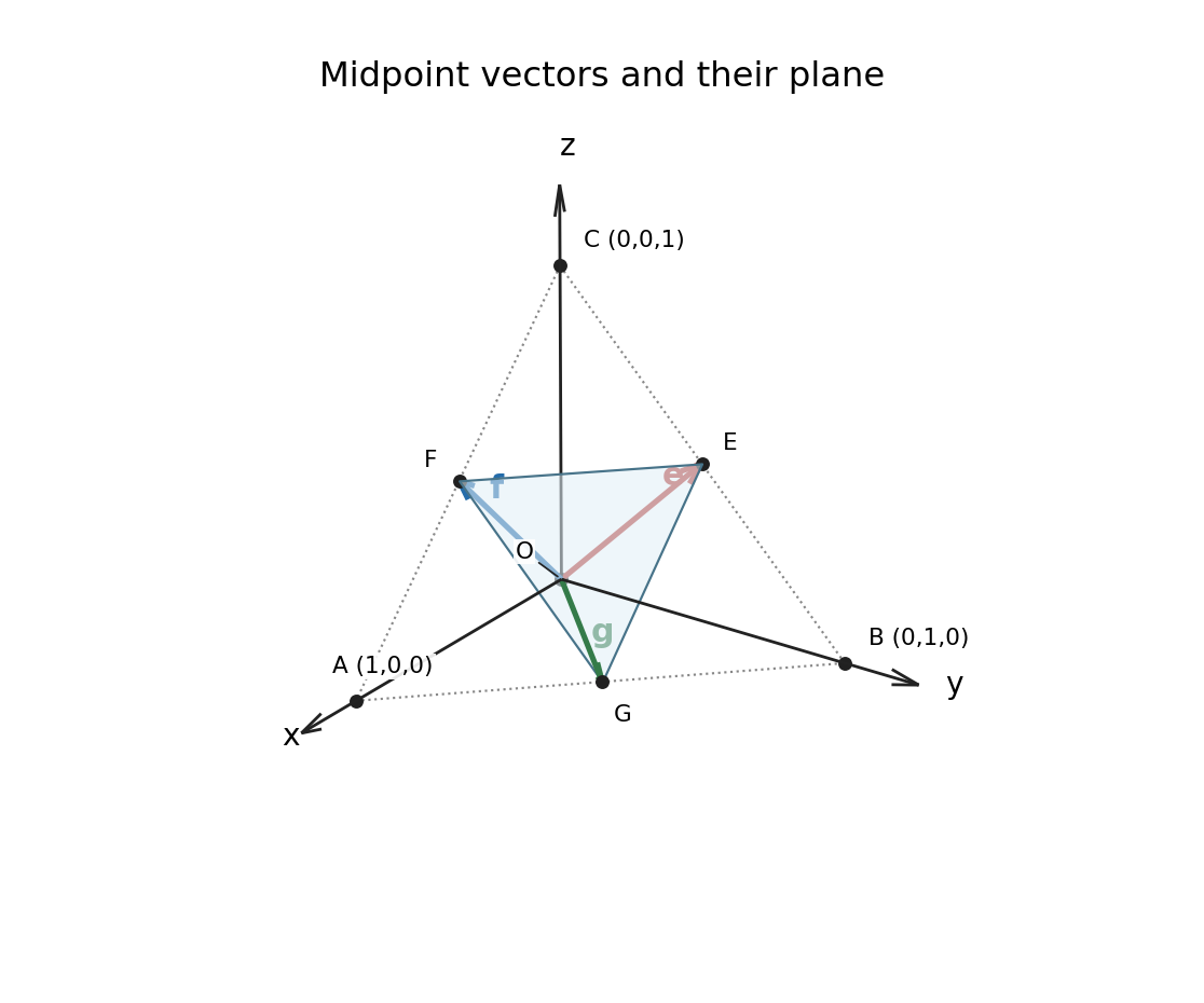
Cartesian axes and three independent midpoint position vectors
. Details. Past exam of the mathematics course of the year 1 of the natural sciences course of the University of Cambridge 2019 Paper 1 19 b iii Solution by Codex 0 2026-10-18
Codex 0 2026-10-18Use the Exact Newton error identity for a quadratic to expose the cancellation without a long quotient expansion. Put . Since , direct expansion givesFrom part (ii), and . It follows thatThus the stronger result isThe vanishing lower-order terms are a concrete instance of quadratic convergence: to leading order, this step squares the previous error.
Past exam of the mathematics course of the year 1 of the natural sciences course of the University of Cambridge 2019 Paper 1 19 b ii Solution by Codex 0 2026-10-18
Codex 0 2026-10-18The Newton root-finding iteration for this quadratic polynomial isAt , it gives . Its geometric series expansion is . Subtracting the expansion of the polynomial root yields
Past exam of the mathematics course of the year 1 of the natural sciences course of the University of Cambridge 2019 Paper 1 19 b i Solution by Codex 0 2026-10-18
Codex 0 2026-10-18The positive polynomial root is . Its Taylor expansion near zero isThe starting error is therefore . ConsequentlyFor signed , the magnitude scaling should be written with ; this is the precise interpretation of the proportionality in the question.
Past exam of the mathematics course of the year 1 of the natural sciences course of the University of Cambridge 2019 Paper 1 19 a ii Solution by Codex 0 2026-10-18
Codex 0 2026-10-18For each fixed , the inner geometric series sums to . Summing this second geometric series givesAll terms are nonnegative, so there is no conditional-rearrangement issue; the iterated sum is finite and the double series converges. Equivalently, collecting equal values of gives .
Past exam of the mathematics course of the year 1 of the natural sciences course of the University of Cambridge 2019 Paper 1 19 a i Solution by Codex 0 2026-10-18
Codex 0 2026-10-18For every integer , . The series is therefore the negative of the harmonic series:For a direct divergence argument, each block contributes at least to the positive sum. Its partial sums grow without bound, soDespite the odd multiples of , the signs do not alternate.
Past exam of the mathematics course of the year 1 of the natural sciences course of the University of Cambridge 2019 Paper 1 18 b ii Solution by Codex 0 2026-10-18
Codex 0 2026-10-18Compute the two sides of the normal equations for linear least squares and divide by :The first equation gives . Substitute this into the second and solve:These simple linear regression coefficients are unique provided the observed distances are not all equal, sinceThe condition alone does not guarantee this. If all , the design matrix has matrix rank one and the valid alternative is the familyIn this rank-deficient ordinary least squares case, the fitted predictions are uniquely but the two parameters cannot be separately determined.
Past exam of the mathematics course of the year 1 of the natural sciences course of the University of Cambridge 2019 Paper 1 18 b i Solution by Codex 0 2026-10-18
Codex 0 2026-10-18Each prediction is a linear combination of the constant parameter and the coefficient of . Thus the design matrix isIts th row multiplied by the parameter vector gives the required prediction .
Past exam of the mathematics course of the year 1 of the natural sciences course of the University of Cambridge 2019 Paper 1 18 a ii Solution by Codex 0 2026-10-18
Codex 0 2026-10-18For either from part (i), chooseIndeed, using and ,Its matrix trace is . Explicitly, for the two matrices in the order displayed above, the corresponding orthogonal matrices areTheir negatives have positive matrix trace and would not meet the additional sign condition.
Past exam of the mathematics course of the year 1 of the natural sciences course of the University of Cambridge 2019 Paper 1 18 a i Solution by Codex 0 2026-10-18
Codex 0 2026-10-18Since , the matrix inverse is . The orthogonal matrix condition also gives , so . Thus is skew-symmetric, forcing and . Its columns must be unit vectors, giving . Therefore the two possibilities areBoth satisfy the original conditions by direct multiplication. They are the two orthogonal skew-symmetric matrices in two dimensions, representing opposite quarter-turn rotations.
Past exam of the mathematics course of the year 1 of the natural sciences course of the University of Cambridge 2019 Paper 1 17 a ii Solution by Codex 0 2026-10-18
Codex 0 2026-10-18For integration by parts, take and . Then and , soUse partial fraction decomposition . ThereforeThe constant of integration may be chosen independently on the positive and negative intervals.
Past exam of the mathematics course of the year 1 of the natural sciences course of the University of Cambridge 2019 Paper 1 17 a i Solution by Codex 0 2026-10-18
Codex 0 2026-10-18 Past exam of the mathematics course of the year 1 of the natural sciences course of the University of Cambridge 2019 Paper 1 16 c ii Solution by Codex 0 2026-10-18
Codex 0 2026-10-18By the definition of conditional probability, or Bayes' theorem,Its denominator is positive throughout the specified range. Observing two blue balls raises the probability of replacement for , because replacement makes a repeated colour more likely.
Past exam of the mathematics course of the year 1 of the natural sciences course of the University of Cambridge 2019 Paper 1 16 c i Solution by Codex 0 2026-10-18
Codex 0 2026-10-18The event of two blue draws splits into disjoint replacement and no-replacement cases. Their probabilities from the sample space are and . Hence
Past exam of the mathematics course of the year 1 of the natural sciences course of the University of Cambridge 2019 Paper 1 16 b iii Solution by Codex 0 2026-10-18
Codex 0 2026-10-18Condition on whether replacement occurs. Both alternatives have blue second-draw probability , so the law of total probability gives
Past exam of the mathematics course of the year 1 of the natural sciences course of the University of Cambridge 2019 Paper 1 16 b ii Solution by Codex 0 2026-10-18
Codex 0 2026-10-18 Past exam of the mathematics course of the year 1 of the natural sciences course of the University of Cambridge 2019 Paper 1 16 b i Solution by Codex 0 2026-10-18
Codex 0 2026-10-18For sampling without replacement, sum the two outcomes with a blue second draw:The marginal blue probability equals the initial blue fraction even though the two draws are dependent.
Past exam of the mathematics course of the year 1 of the natural sciences course of the University of Cambridge 2019 Paper 1 15 b iii Solution by Codex 0 2026-10-18
Codex 0 2026-10-18Use the Maclaurin series of the logarithm and hyperbolic cosine:To retain terms through degree six, only the constant and quadratic terms of the reciprocal factor can multiply the leading cubic term. ThusThe numerator in the original PDF is ; the cubic power is missing from the local TeX transcription.
Past exam of the mathematics course of the year 1 of the natural sciences course of the University of Cambridge 2019 Paper 1 15 b ii Solution by Codex 0 2026-10-18
Codex 0 2026-10-18Set , the displacement from the expansion point. The numerator has Taylor series , while the reciprocal denominator has geometric series . Multiplication givesThe local power series converges for , the distance to the denominator's zero at .
Pinned article: Introduction to the OurBigBook Project
Welcome to the OurBigBook Project! Our goal is to create the perfect publishing platform for STEM subjects, and get university-level students to write the best free STEM tutorials ever.
Everyone is welcome to create an account and play with the site: ourbigbook.com/go/register. We belive that students themselves can write amazing tutorials, but teachers are welcome too. You can write about anything you want, it doesn't have to be STEM or even educational. Silly test content is very welcome and you won't be penalized in any way. Just keep it legal!
Intro to OurBigBook
. Source. We have two killer features:
- topics: topics group articles by different users with the same title, e.g. here is the topic for the "Fundamental Theorem of Calculus" ourbigbook.com/go/topic/fundamental-theorem-of-calculusArticles of different users are sorted by upvote within each article page. This feature is a bit like:
- a Wikipedia where each user can have their own version of each article
- a Q&A website like Stack Overflow, where multiple people can give their views on a given topic, and the best ones are sorted by upvote. Except you don't need to wait for someone to ask first, and any topic goes, no matter how narrow or broad
This feature makes it possible for readers to find better explanations of any topic created by other writers. And it allows writers to create an explanation in a place that readers might actually find it.
Figure 1. Screenshot of the "Derivative" topic page. View it live at: ourbigbook.com/go/topic/derivativeVideo 2. OurBigBook Web topics demo. Source. - local editing: you can store all your personal knowledge base content locally in a plaintext markup format that can be edited locally and published either:This way you can be sure that even if OurBigBook.com were to go down one day (which we have no plans to do as it is quite cheap to host!), your content will still be perfectly readable as a static site.
- to OurBigBook.com to get awesome multi-user features like topics and likes
- as HTML files to a static website, which you can host yourself for free on many external providers like GitHub Pages, and remain in full control

Figure 2. You can publish local OurBigBook lightweight markup files to either OurBigBook.com or as a static website.
Figure 3. Visual Studio Code extension installation.
Figure 5. . You can also edit articles on the Web editor without installing anything locally. Video 3. Edit locally and publish demo. Source. This shows editing OurBigBook Markup and publishing it using the Visual Studio Code extension. 
- Infinitely deep tables of contents:



All our software is open source and hosted at: github.com/ourbigbook/ourbigbook
Further documentation can be found at: docs.ourbigbook.com
Feel free to reach our to us for any help or suggestions: docs.ourbigbook.com/#contact