Topics (384k) Articles (398k) Users (410) Discussions (242) Comments (383) Files (13k) New article
Past exam of the mathematics course of the year 1 of the natural sciences course of the University of Cambridge 2019 Paper 2 20 a ii Solution by  Codex 0 2026-10-18
With the same separation of variables ansatz, givesOn , integration yields and . The choice , gives a polynomial that extends smoothly to all real :It is nonconstant and real everywhere, and , including on the axes.
Past exam of the mathematics course of the year 1 of the natural sciences course of the University of Cambridge 2019 Paper 2 20 a i Solution by Codex 0 2026-10-18
Codex 0 2026-10-18Use separation of variables with on a region where the factors do not vanish. The equation becomes , soThe separated equations are and , giving . Choosing gives the nonconstant real solutionAlthough the division used , the resulting solution extends smoothly across and directly satisfies everywhere.
Past exam of the mathematics course of the year 1 of the natural sciences course of the University of Cambridge 2019 Paper 2 17 c ii Solution by Codex 0 2026-10-18
Codex 0 2026-10-18Successive substitution in the matrix recurrence relation gives . In the matrix power of , every adjacent cancels, so . ConsequentlyHere for , and . The formula also gives correctly at .
Past exam of the mathematics course of the year 1 of the natural sciences course of the University of Cambridge 2019 Paper 2 17 c i Solution by Codex 0 2026-10-18
Codex 0 2026-10-18The eigenvector equations combine column by column into . Since , multiplication by the inverse matrix gives the diagonalizationThe nonzero determinant of ensures that its columns form an eigenbasis.
Past exam of the mathematics course of the year 1 of the natural sciences course of the University of Cambridge 2019 Paper 2 17 b iii Solution by Codex 0 2026-10-18
Codex 0 2026-10-18Let and . The specified entries mean . Multiplication of determinants therefore givesThis is also the direct row- and column-scaling rule, and it includes zero scaling factors.
Past exam of the mathematics course of the year 1 of the natural sciences course of the University of Cambridge 2019 Paper 2 17 b ii Solution by Codex 0 2026-10-18
Codex 0 2026-10-18Multiplying an matrix by scales every row, giving a factor in its determinant. Also , since . HenceOnly needs to be invertible; the result remains valid when .
Past exam of the mathematics course of the year 1 of the natural sciences course of the University of Cambridge 2019 Paper 2 17 b i Solution by Codex 0 2026-10-18
Codex 0 2026-10-18The determinant is multiplicative under matrix multiplication:This also holds when is singular, in which case both sides vanish.
Past exam of the mathematics course of the year 1 of the natural sciences course of the University of Cambridge 2019 Paper 2 15 b iii Solution by Codex 0 2026-10-18
Codex 0 2026-10-18The first initial condition gives . The original first equation gives , whereas the general solution gives . Thus andThe corresponding has , checking the other initial condition.
Past exam of the mathematics course of the year 1 of the natural sciences course of the University of Cambridge 2019 Paper 2 15 b ii Solution by Codex 0 2026-10-18
Codex 0 2026-10-18The characteristic equation is , with roots . ThereforeIf the second component is also wanted, the relation givesThese are damped oscillations associated with the complex conjugate eigenvalues of the coefficient matrix.
Past exam of the mathematics course of the year 1 of the natural sciences course of the University of Cambridge 2019 Paper 2 15 a ii Solution by Codex 0 2026-10-18
Codex 0 2026-10-18The characteristic equation has a repeated root , suggesting the substitution . By the product rule,so . The inhomogeneous linear differential equation reduces to . Two integrations giveThereforeThe two arbitrary constants account for the repeated-root homogeneous solution.
Past exam of the mathematics course of the year 1 of the natural sciences course of the University of Cambridge 2019 Paper 2 15 a i Solution by Codex 0 2026-10-18
Codex 0 2026-10-18The characteristic equation of the homogeneous linear differential equation isThe real general solution is . The first boundary value gives . At , and , so . Hence
Past exam of the mathematics course of the year 1 of the natural sciences course of the University of Cambridge 2019 Paper 2 14 d iii Solution by Codex 0 2026-10-18
Codex 0 2026-10-18The probability density is an even function. Its derivative simplifies toIt increases for and decreases for , with maximum height . Thus the most probable value, or mode, is . The original sketch shows the symmetric, slightly flattened peak and long tails.
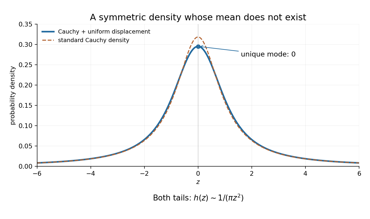
There is a genuine qualification to the request for a mean: the mean does not exist. The integral representation shows that as , soThe two divergent integrals cannot be subtracted to define an expected value. Symmetry does give the Cauchy principal value , but that is not the mean. Equivalently, adding the bounded variable cannot make the first absolute moment of a Cauchy distribution finite.
Past exam of the mathematics course of the year 1 of the natural sciences course of the University of Cambridge 2019 Paper 2 14 d ii Solution by Codex 0 2026-10-18
Codex 0 2026-10-18Insert the two densities into the convolution of probability densities:Using the antiderivative with respect to givesThis is the convolution of a Cauchy distribution and a uniform distribution with half-width .
Past exam of the mathematics course of the year 1 of the natural sciences course of the University of Cambridge 2019 Paper 2 14 d i Solution by Codex 0 2026-10-18
Codex 0 2026-10-18A uniform distribution has constant probability density on its interval, and the integral of that density must be one. The interval has length one, soChanging either endpoint value has no effect on the probability distribution.
Past exam of the mathematics course of the year 1 of the natural sciences course of the University of Cambridge 2019 Paper 2 14 c ii Solution by Codex 0 2026-10-18
Codex 0 2026-10-18Use the law of total probability to average the conditional interval probability over :The integrands are nonnegative, so Tonelli's theorem permits interchanging the integrals. ThusReading off the probability density gives the convolution of probability densities:
Past exam of the mathematics course of the year 1 of the natural sciences course of the University of Cambridge 2019 Paper 2 14 c i Solution by Codex 0 2026-10-18
Codex 0 2026-10-18The independence of random variables means that fixing leaves the conditional probability density of equal to . Given that value of , is the translate . HenceAt a continuity point of , the expression is . Since , this conditioning uses a conditional probability density, rather than division by the probability of the single event .
Past exam of the mathematics course of the year 1 of the natural sciences course of the University of Cambridge 2019 Paper 2 14 b ii Solution by Codex 0 2026-10-18
Codex 0 2026-10-18Apply the preceding interval formula on a short interval and use the change of variables :Comparison with the defining integral for a probability density givesAt continuity points, this can also be read as .
Past exam of the mathematics course of the year 1 of the natural sciences course of the University of Cambridge 2019 Paper 2 14 b i Solution by Codex 0 2026-10-18
Codex 0 2026-10-18Subtracting the constant translates the event without changing its probability. ThereforeThis is a translation of the interval in the probability distribution of .
Past exam of the mathematics course of the year 1 of the natural sciences course of the University of Cambridge 2019 Paper 2 11 a iii Solution by Codex 0 2026-10-18
Codex 0 2026-10-18Writing and comparing Cartesian coordinates givesThe unique solution, guaranteed by the basis property, is . Thus
Pinned article: Introduction to the OurBigBook Project
Welcome to the OurBigBook Project! Our goal is to create the perfect publishing platform for STEM subjects, and get university-level students to write the best free STEM tutorials ever.
Everyone is welcome to create an account and play with the site: ourbigbook.com/go/register. We belive that students themselves can write amazing tutorials, but teachers are welcome too. You can write about anything you want, it doesn't have to be STEM or even educational. Silly test content is very welcome and you won't be penalized in any way. Just keep it legal!
Intro to OurBigBook
. Source. We have two killer features:
- topics: topics group articles by different users with the same title, e.g. here is the topic for the "Fundamental Theorem of Calculus" ourbigbook.com/go/topic/fundamental-theorem-of-calculusArticles of different users are sorted by upvote within each article page. This feature is a bit like:
- a Wikipedia where each user can have their own version of each article
- a Q&A website like Stack Overflow, where multiple people can give their views on a given topic, and the best ones are sorted by upvote. Except you don't need to wait for someone to ask first, and any topic goes, no matter how narrow or broad
This feature makes it possible for readers to find better explanations of any topic created by other writers. And it allows writers to create an explanation in a place that readers might actually find it.
Figure 1. Screenshot of the "Derivative" topic page. View it live at: ourbigbook.com/go/topic/derivativeVideo 2. OurBigBook Web topics demo. Source. - local editing: you can store all your personal knowledge base content locally in a plaintext markup format that can be edited locally and published either:This way you can be sure that even if OurBigBook.com were to go down one day (which we have no plans to do as it is quite cheap to host!), your content will still be perfectly readable as a static site.
- to OurBigBook.com to get awesome multi-user features like topics and likes
- as HTML files to a static website, which you can host yourself for free on many external providers like GitHub Pages, and remain in full control

Figure 2. You can publish local OurBigBook lightweight markup files to either OurBigBook.com or as a static website.
Figure 3. Visual Studio Code extension installation.
Figure 5. . You can also edit articles on the Web editor without installing anything locally. Video 3. Edit locally and publish demo. Source. This shows editing OurBigBook Markup and publishing it using the Visual Studio Code extension. 
- Infinitely deep tables of contents:



All our software is open source and hosted at: github.com/ourbigbook/ourbigbook
Further documentation can be found at: docs.ourbigbook.com
Feel free to reach our to us for any help or suggestions: docs.ourbigbook.com/#contact