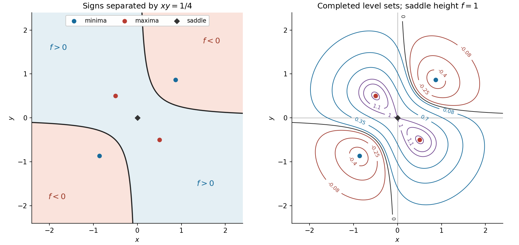
The completed contour plot is shown in the right-hand panel. Its geometry follows from the symmetries $f(-x,-y)=f(x,y)$ and $f(y,x)=f(x,y)$, together with $f\to 0$ as $x^2+y^2\to \infty$. For orientation, the two local minima have value $-2e^{-3/2}$, the two local maxima have value $2e^{-1/2}$, and the saddle point has value one.

Negative level sets between $-2e^{-3/2}$ and zero form separate closed curves around the two local minima in the first and third quadrants. Positive level sets below one form a single closed curve enclosing the origin and both local maxima. At level one, a critical level set crosses itself at the origin and surrounds the two local maxima in two lobes. Between one and $2e^{-1/2}$, the level sets split into separate closed curves around those local maxima. The zero level set remains the two unbounded branches $xy=1/4$.

Near the origin, the Taylor expansion is $f=1-x^2-4xy-y^2+O((x^2+y^2{)}^2)$. Consequently the crossing directions at the saddle height satisfy $y=(-2\pm \sqrt{3})x$, giving the local shape of the critical level set.

Evaluate the Hessian matrix at the five stationary points. At the origin it iswhose eigenvalues are $-6$ and $2$, so the origin is a saddle point. At the two points with $x=y=\pm \sqrt{3}/2$,whose eigenvalues are $12e^{-3/2}$ and $8e^{-3/2}$. Both are positive, so these are strict local minima. At the two points with $x=-y=\pm 1/2$,whose eigenvalues are $-8e^{-1/2}$ and $-4e^{-1/2}$. Both are negative, so these are strict local maxima. In summary,The quadratic changes along the orthogonal directions $(1,1)$ and $(1,-1)$ also provide a direct justification of these classifications.

Set both components of the gradient to zero. After dividing out the nonzero exponential, they are equivalent toAdding and subtracting gives $(x+y)(3-4xy)=0$ and $(x-y)(1+4xy)=0$. If $x=y$, the first equation reduces to $x(3-4x^2)=0$, giving the origin and the two diagonal points. If $x=-y$, it reduces to $x(4x^2-1)=0$, giving the origin and the two opposite-diagonal points. The alternative simultaneous values $xy=3/4$ and $xy=-1/4$ are incompatible, so these cases exhaust the possibilities. Thus the five stationary points areThey are marked in both panels of the figure.

The sign of $f$ is the sign of $1-4xy$. ThereforeThe positive region includes both coordinate axes, the second and fourth quadrants, and the portions of the first and third quadrants on the origin side of the hyperbola. The two negative regions lie beyond its branches. The left-hand panel shows these regions; its markers locate the stationary points calculated next.

The exponential function is strictly positive, so the zero level set is determined entirely by its prefactor:This is a rectangular hyperbola with branches in the first and third quadrants.

For real solutions with $x>0$, the square root requires $y\ge 0$. First retain the solution $y\equiv 0$, which would be lost by dividing by a square root of $y$.

For $y>0$, use the homogeneous first-order differential equation substitution $v=\sqrt{y/x}>0$, so $y=x{v}^2$, $\sqrt{xy}=xv$ and $y^{\prime }=v^2+2xv{v}^{\prime }$. The equation becomesThis is now a separable differential equation. Integration gives $-2/v+2\ln v=-\ln x+C$. Since $x{v}^2=y$, the positive solutions satisfyThe implicit family is sufficient here because only parts (a) and (b) request an explicit expression. It also shows why the nonnegative choice of $v$ matters: $\sqrt{xy}$ denotes the positive square root.

The original PDF has $8y^3-4x$ in the denominator and $dy/dx$ on the left. Rearrange it into the differential formThe cross partial derivatives of its coefficients are both four, so it is an exact differential form. Integrating its first coefficient in $x$ gives a potential $F=\frac{5}{2}{x}^2+4xy+h(y)$. Matching $F_y=4x-8y^3$ gives $h(y)=-2y^4$. Therefore an implicit general solution isDifferentiating verifies $y^{\prime }=(5x+4y)/(8y^3-4x)$. A solution graph is understood only on intervals where its denominator is nonzero; the printed quotient does not define a derivative when $8y^3=4x$.

Rewrite the linear ordinary differential equation as $y^{\prime }+y=e^{3x}$. Multiplication by its integrating factor $e^x$ gives $(e^{x}y{)}^{\prime }=e^{4x}$. Integrating yieldsThe general solution consists of this particular solution and the homogeneous solution $C{e}^{-x}$.

For $x\ne 0$, divide by $x^2$ to obtain $y^{\prime }+y/x=1/x^2$, a first-order linear ordinary differential equation. An integrating factor is $x$ on either interval not crossing zero, since the product rule givesIntegration and division by $x$ give the explicit general solutionThe original equation would read $0=1$ at zero, so no solution can include that point.

By De Moivre's theorem, $\cos 5\theta$ is the real part of $(\cos \theta +i\sin \theta {)}^5$. Writing $c=\cos \theta$ and $s=\sin \theta$, the binomial theorem givesUse the Pythagorean trigonometric identity $s^2=1-c^2$ and expand:Therefore

Using the exponential definition of hyperbolic tangent, set $q=e^{2z}$:Here $q+1=1-i\ne 0$, so the resulting points are not poles. Taking all values of the complex logarithm gives $2z=i(-\pi /2+2\pi k)$. ThusEquivalently $\tanh (iu)=i\tan u$, so these are exactly the imaginary-axis solutions of $\tan u=-1$.

The factor $1+i$ has modulus $\sqrt{2}$ and principal argument $\pi /4$. Multiplication by $e^{i\pi /6}$ adds $\pi /6$ to its complex argument, while the real factor $1/2$ halves its modulus. HenceTaking the principal logarithm for $w$ givesThis complex number lies in the second quadrant. Its modulus follows from the sum of squared components, and its principal argument follows by the second-quadrant correction:All arguments of this fixed $w$ add integer multiples of $2\pi$ to the displayed one.

If $\ln z$ is interpreted as the multivalued complex logarithm, there is instead a family $w_k=-a+i{b}_k$, where $a=\frac{1}{2}\ln 2>0$ and $b_k=5\pi /12+2\pi k$. Then $|w_k|=\sqrt{a^2+b_k^2}$, and the principal argument is $\pi -\arctan (b_k/a)$ for $b_k>0$, or $-\pi -\arctan (b_k/a)$ for $b_k<0$. This records the logarithm-branch choice that the paper leaves implicit.

The two derivatives are $3x^2+3$ and $6x$, both equal to six at $x=1$. Their common tangent line through $(1,4)$ is $y-4=6(x-1)$, or $y=6x-2$. Setting $x=0$ gives its intersection with the vertical axis:

Equating the two polynomials gives $x^3-3x^2+3x-1=(x-1{)}^3=0$. Thus the only intersection has $x=1$ and $y=4$:

Substitution in the logarithmic expression gives $x\simeq 23.8/0.301=79.069\dots$. To two significant figures,