The remaining proper subgroups areTheir orders are respectively one, three, six, four and six. The order-four groups are Klein four-groups; the last two are dihedral groups of order six, isomorphic to $S_3$.

For completeness, if $H$ contains a reflection, write $H\cap ⟨g⟩=⟨g^d⟩$ with $d\mid 6$. Any other reflection differs from a chosen $g^{j}h$ by an element of this rotational subgroup, so $H=⟨g^d,g^{j}h⟩$ with $j$ specified modulo $d$. The choices $d=1,2,3,6$ give respectively the whole group, the two order-six groups, the three order-four groups and the six reflection groups already listed. This proves there are no omitted subgroups.

Thus there are eight remaining proper subgroups. The printed count nine includes one too many; nine would be correct if the whole group were included with these remaining subgroups. Altogether $G$ has sixteen subgroups, fifteen proper.

The involutions in an even dihedral group are the half-turn $g^3$ and the six reflections $g^{j}h$. Thus the seven order-two subgroups areThe half-turn is central, so only $⟨g^3⟩$ is normal. Indeed $g(g^{j}h)g^{-1}=g^{j+2}h$, a different reflection; an order-two subgroup has only one nonidentity element, so each reflection subgroup fails the normal subgroup condition.

Introduce the velocity variable $v=\dot{x}$. The second-order differential equation becomes the autonomous planar systemA critical point of a dynamical system is a point where both components of the vector field vanish: here $v=0$ and $f(x,0)=0$. It is a stationary solution in the phase plane. The Jacobian matrix at each such point gives the local linear stability of a planar equilibrium. For the equations below, a conserved energy also determines the nonlinear phase portrait; this is important because purely imaginary eigenvalues alone do not generally prove that an equilibrium is a center equilibrium.

For random variables with finite second moments, their covariance isThe Cauchy-Schwarz inequality ensures the product is integrable under this hypothesis. More generally the definition works whenever the displayed expectations exist. Assertions about arbitrary random variables below are understood on this domain: without suitable moments a covariance need not be defined at all.

For the final limit, near zero $\cos x>0$, so the real logarithm is well defined. First apply the proved rule to $\tan x/x$ on the right: its derivative ratio is ${\sec }^{2}x\to 1$. Next apply it to $\log (\cos x)/x^2$; the derivative ratio isThe original quotient is even, so the left limit equals the right limit. Consequently

Now impose the stated zero endpoint values and nonvanishing assumptions near $a$. For each $x\in (a,a+\delta )$, applying the proved identity on $[a,x]$ gives some $c_x\in (a,x)$ such thatAs $x\downarrow a$, every possible $c_x$ also tends to $a$. Explicitly, for any $\epsilon >0$, choose a right neighborhood of $a$ where $|f^{\prime }/g^{\prime }-L|<\epsilon$. If $x$ lies in it, so does $c_x$, and therefore $|f(x)/g(x)-L|<\epsilon$. This proves the endpoint zero-over-zero form of L'Hôpital's rule:No continuity of either derivative is required, only their ratio limit and the given nonvanishing conditions.

For the two-function assertion, defineThis function has the required continuity and differentiability and satisfies $H(a)=H(b)=0$. Rolle's theorem therefore gives $c$ withThis proves the Cauchy mean value theorem even when either endpoint increment vanishes; no division was used.

Rolle's theorem states that if a real function $h$ is continuous on $[a,b]$, differentiable on $(a,b)$, with $a<b$ and $h(a)=h(b)$, then some $c\in (a,b)$ satisfies $h^{\prime }(c)=0$.

The strong plume's outgoing flux equals the total lower-layer supply, $Q_2(h_2)=Q$. Apply the additional closure in this part and the lower-layer balance from part (b):Dividing by $C{B}_2^{1/3}{h}_1^{5/3}$ givessoFor $0<\psi <1$ this puts the second matching level above the first. It tends to one as $\psi \to 0$ and to $2^{2/5}$ as $\psi \to 1$. At the latter endpoint the two warm layers already have identical density, so $h_2$ is only a formal matching label, not a distinct observable interface. The expression follows from the stipulated closure; modeling the actual plume in the changed ambient requires the matched continuation discussed in part (d).

Above $h_1$, plume 2 entrains middle-layer fluid rather than the original ambient. That fluid is already warm and light, so the plume's buoyancy relative to its surroundings is reduced. Its pre-interface density contrast and zero-source pure plume formula cannot simply be continued unchanged through the interface.

A consistent model treats the middle layer as a uniform new ambient, assumes a sharp interface and weak overall density differences, and carries the incident volume and momentum fluxes continuously across it. The relative buoyancy flux immediately above the interface isContinue an entraining plume model from these nonzero incident fluxes, using buoyancy measured relative to the middle layer. In that uniform layer the relative buoyancy flux is conserved, while entrainment raises the absolute buoyancy carried relative to the outside environment. This is generally a finite-flux or forced plume continuation, not a newly reset point-source similarity solution. A virtual-origin approximation can be used only after matching its fluxes appropriately.

At its matching level $h_2$, the plume density reaches the upper-layer density; it spreads and detrains, with possible finite-momentum overshoot. The model neglects mutual plume entrainment, wall heat transfer, interface thickness and detailed intrusion dynamics, and assumes each ambient layer is well mixed. In the equal-source limit $B_2^{+}=0$, the continuation is a neutrally buoyant momentum-driven flow, emphasizing why the upper interface loses its independent density meaning.

Put $\psi =B_1/B_2$. The middle layer matches the density of plume 1 at $h_1$, so $g_1^{\prime }=B_1/q_1$. The upper layer exports both sources, so $g_2^{\prime }=(B_1+B_2)/Q$. With $Q=q_1+q_{21}$ and $q_{21}/q_1={\psi }^{-1/3}$, the two-plume three-layer displacement ventilation density ratio isThe driving head can therefore be rewritten as $\mathcal{H}=g_2^{\prime }\mathcal{L}$, whereCombining $Q^2=(A^{\ast }{)}^2{g}_2^{\prime }\mathcal{L}$ with $g_2^{\prime }Q=B_2(1+\psi )$ gives $Q^3=(A^{\ast }{)}^2{B}_2(1+\psi )\mathcal{L}$. But $Q^3=C^3{B}_2(1+{\psi }^{1/3}{)}^3{h}_1^5$, and henceThe square root requires a positive remaining buoyancy head.

As $\psi \to 0$, the weak source vanishes and $g_1^{\prime }/g_2^{\prime }\to 0$: the middle and lower layers have the same density, leaving a single physical interface at $h_2$. The old $h_1$ no longer marks an independent density interface. The single-plume two-layer model is the meaningful limit; the additional closure in part (e) also gives $h_2/h_1\to 1$.

As $\psi \to 1$, the density ratio tends to one, so the middle and upper layers merge. There is then a single physical lower interface $h_1$, fed by two equal, separate plumes. The area prefactor tends to two and the head reduces to $g^{\prime }(H-h_1)$. The mathematical label $h_2$ ceases to identify a distinct density interface, so a finite limiting value assigned to it by an extra closure is not evidence for three distinct layers. Two separate equal plumes entrain more than one coincident plume of combined source strength; the distinction survives after the layers merge.

Let $g_i^{\prime }=g\Delta {\rho }_i/\rho$ denote the density deficit of each warm layer relative to outside. The integrated hydrostatic driving head isThe same pair of orifice laws therefore givesBoth plumes remove fluid from the lower layer. If $q_1=C{B}_1^{1/3}{h}_1^{5/3}$ and $q_{21}=C{B}_2^{1/3}{h}_1^{5/3}$ are their fluxes at its upper interface, lower-layer conservation also givesIn steady state the weak plume supplies the middle layer, while the strong plume entrains that supply above $h_1$ and carries the total volume into the upper layer. Consequently $Q_2(h_2)=Q$ and $g_2^{\prime }Q=B_1+B_2$. These balances assume the plumes remain spatially separate and wall heat loss is negligible.

Assume Boussinesq approximation, no wind, a uniform exterior, negligible source volume, sharp well-mixed internal layers, point-source pure plume entrainment and thin openings represented by discharge coefficients $C_b,C_t$. Let $g_1^{\prime }=g\Delta {\rho }_1/\rho$ be the upper-layer reduced gravity. Steady volume conservation makes the magnitudes of inlet and outlet flow equal to $Q$.

If the opening pressure drops are $\Delta p_b$ and $\Delta p_t$, the orifice laws and hydrostatic pressure difference giveDefine the reduced area byThen the throughflow in this displacement ventilation model isLower-layer conservation requires $Q=Q_p(h_1)=C{B}_1^{1/3}{h}_1^{5/3}$. Global buoyancy conservation gives $g_1^{\prime }Q=B_1$. Eliminating $Q,g_1^{\prime }$ yieldsThis uniquely determines an interface height between zero and $H$ for a given positive area parameter. Opening area controls the nondimensional height; source strength controls the density contrast and flow magnitude. Factors of two depend on the stated effective-area convention, which has been fixed explicitly here.

The flux solution gives $w=M/Q=s{z}^{-1/3}$, while $b^2=Q^2/(\rho M)$. ThusAt $z=z_b$, $\rho ={\rho }_0/2$, $T=2T_0$ and $g^{\prime }=g/2$. This height marks the transition between a strongly non-Boussinesq near-source plume and the dilute far-field plume. For $z\gg z_b$, $b\sim dz$ and $g^{\prime }\sim g(z_b/z{)}^{5/3}=(4s^2/3)z^{-5/3}$, recovering the Boussinesq solution. For $z\ll z_b$, $b\sim d{z}_b^{5/6}{z}^{1/6}$, $g^{\prime }\to g$ and $\rho \propto z^{5/3}$.

The ideal point-source limit still has a divergent velocity and temperature; it is not a literal resolved finite burner. In particular, zero source mass flux does not imply zero physical hot-gas volume flux: $w{b}^2$ tends to $B/g$ in this limiting solution. Source size, compressibility and heat transfer impose additional near-source limits on the model.

From the definitions of mass and momentum fluxes,The density relation follows by solving the conserved-buoyancy identity in the preceding part. Hence $wb\sqrt{\rho }=\sqrt{M}$ andThe second equality uses $B=g({\rho }_0-\rho )Q/({\rho }_0\rho )$ and $b^2=Q^2/(\rho M)$.

Set $q=Q/{\rho }_0$ and $m=M/{\rho }_0$. The equations become $q^{\prime }=2\alpha \sqrt{m}$, $m^{\prime }=Bq/m$, exactly the same flux system as for the pi-suppressed Boussinesq pure plume. For the heated point source take zero initial mass and momentum flux and the finite conserved heat/buoyancy supply. DefineThe resulting mass and momentum fluxes areSubstituting $Q$ into the density relation gives the non-Boussinesq pure-plume density transitionThe two expressions for $z_b$ agree because $B=4d^2{s}^3/3$. Density increases from the very dilute near-source regime toward the ambient value as entrainment increases the mass flux.

The mass and heat entrainment equations immediately giveUse the specified relation $\rho T={\rho }_0{T}_0=\beta$. ThenMeanwhile the kinematic buoyancy flux isSince $T_0$, ${\rho }_0$ and $c_p$ are constant,Thus conservation is a consequence of conserved excess heat in this ideal-gas, uniform-ambient model, not merely an assumption that arbitrary non-Boussinesq buoyancy fluxes are conserved in every environment.

Use the flux normalization of the supplied equations, with the common factor $\pi$ suppressed. Put $q=w{b}^2$, $m=w^2{b}^2$ and $B_0=g^{\prime }q$. The top-hat plume model reduces toEliminate height to obtain $dm/dq=B_{0}q/(2\alpha m^{3/2})$. Integrating with zero source volume and momentum flux gives the pure plume balanceEquivalently, seek $b=dz$ and $w=s{z}^{-1/3}$. The volume balance gives $d=6\alpha /5$, and the momentum and buoyancy balances give $g^{\prime }=(4s^2/3)z^{-5/3}$ and $B_0=4d^2{s}^3/3$. ThusA finite source replaces the singular point origin by a plume virtual origin and source conditions. The Boussinesq approximation requires the fractional density difference to be small, so density can be replaced by ambient density in inertia and entrainment while retaining the small difference in buoyancy. In this solution it requires $g^{\prime }/g\ll 1$. The approximation necessarily fails sufficiently near the ideal point source, where $g^{\prime }$ diverges, and can also fail for strongly heated or otherwise large-density-contrast sources. The similarity solution is appropriate farther away once entrainment has diluted the anomaly, assuming a uniform ambient, constant entrainment coefficient and negligible confinement, heat loss and stratification.

Because $\zeta <\eta \le h(x)$, the lower layer is saturated along the entire barrier. Both layers have the same horizontal head gradient but different Darcy velocities. Integrating their conductivity over the actual cross-section gives the transmissivityThe total discharge is $Q=-\mathcal{T}(h)h_x$. Hence $QL={\int }_{\eta }^H\mathcal{T}(h)dh$, givingThis is a parallel-layer conductivity integral, not a series-resistance average: the layers share the horizontal pressure drop. It reduces to the previous result when $k_1=k_2$. The assumption $\zeta <\eta$ is important; if the downstream free surface cuts the lower layer, the transmissivity and its head integration must be split into different saturation regimes.

Assume quasi-steady saturated Darcy flow, hydrostatic pore pressure, a long shallow barrier, isotropic intrinsic permeability of a porous medium $k$, an impermeable lined base, and negligible capillarity. Maintain upstream and downstream free-surface heads at $H$ and $\eta <H$. The Dupuit approximation neglects vertical velocity except in small entrance/exit regions. Let $\mu$ be the fluid's dynamic viscosity and $K=k\rho g/\mu =kg/\nu$ its hydraulic conductivity.

Since the pressure is $p=\rho g(h(x)-z)$, the superficial Darcy velocity is $v_D=-K{h}_x$, uniform with depth at fixed $x$. Integrating over the printed channel width givesThe steady discharge is constant, so integration with the two head boundary values gives Dupuit flow in a channel with cubic wetted area:Here $Q$ is total volume per time, including the changing channel width. The pore-space mean speed is $v_p=v_D/\varphi =Q/[\varphi A(h)]$. Thus porosity affects storage and pore transit time but does not separately multiply this steady discharge when $k$ is the intrinsic permeability in Darcy's law. If “permeability” is instead supplied as hydraulic conductivity, use that value directly for $K$. An exact seepage-face/free-boundary calculation near the outlet would go beyond the shallow Dupuit model.

Treat the newly placed sand barrier as impermeable during the initial release. The downstream isolated reservoir occupies $-\ell <x<0$ with depth $H$ and has finite volume $\alpha H^3\ell /3$. The remaining upstream water stays behind the barrier; it does not continuously feed the released region. Assume $\ell \gg H$ so that the shallow-water approximation is appropriate.

Until the rarefaction head reaches the barrier atthe previous dam-break solution is unchanged on the released side. The wall imposes $u(-\ell ,t)=0$. After $t_1$, a reflected downstream family adjusts the flow near the wall. It is a lowering/depletion adjustment, not a new upstream supply. The upstream depth decreases, the finite water volume spreads downstream, and the unmodified simple-wave region shrinks relatively.

The leading characteristic of this adjustment can be determined exactly without solving the whole reflected region. In the still-unmodified fan,Integrating gives the finite-reservoir reflection of a cubic-area dam-break rarefaction:The solution to the right of this curve is still the original fan. Crucially $x_f-x_r=7c_0{t}_1^{2/7}{t}^{5/7}>0$ at every finite time. Therefore the ideal inviscid dry tip remains at $x_f=6c_{0}t$: finite reservoir volume does not by itself justify an immediate change to that front law. Only a vanishingly small amount of fluid occupies its very thin forward tail at late times. Bottom drag, leakage or other front physics changes this conclusion.

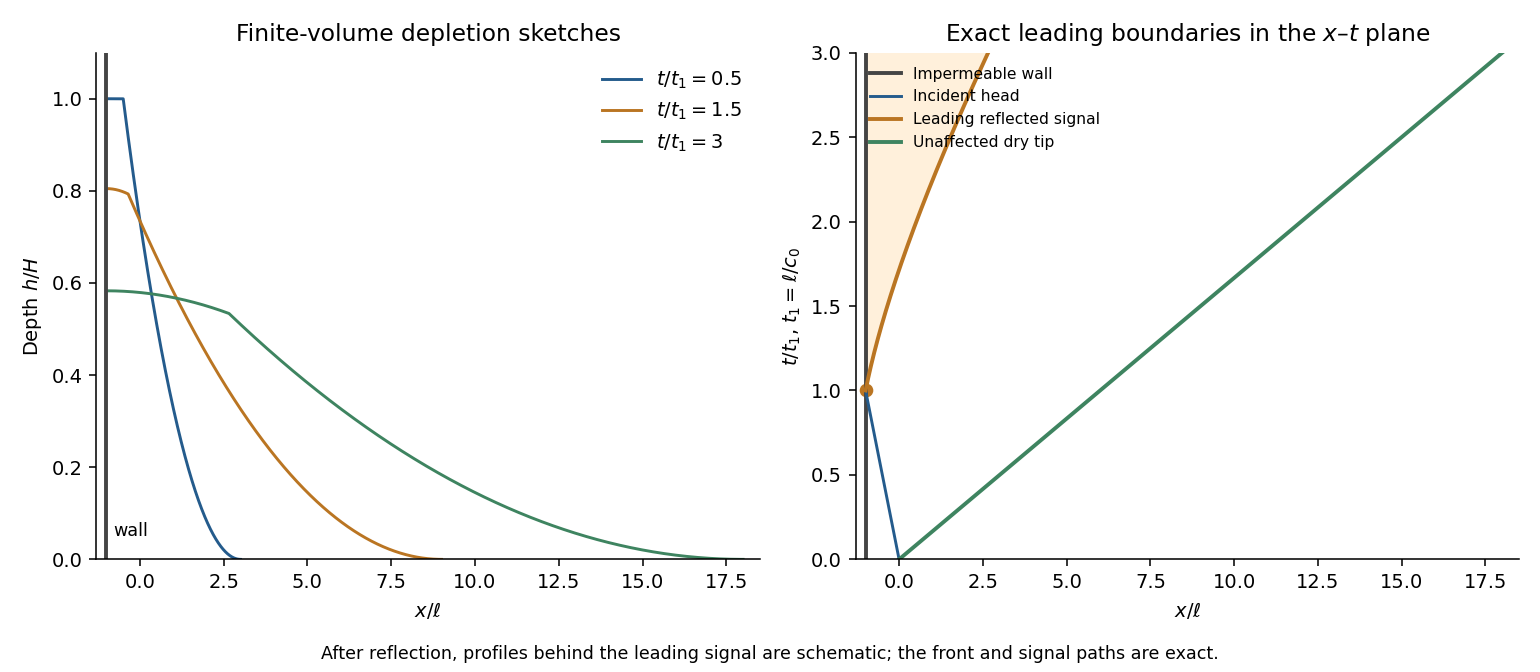
The profiles behind the reflected edge are schematic; there the two characteristic families interact and the original one-invariant fan no longer supplies the complete fields. The x–t diagram distinguishes the wall, the incident head, the exact reflected leading edge and the unaffected dry-tip trajectory.