A stationary distribution is a nonnegative row vector $\pi$ with $\pi P=\pi$ and ${\sum }_i{\pi }_i=1$. The balance equations giveThe first yields ${\pi }_1={\pi }_4$. Substitution into the middle pair yields ${\pi }_2=3{\pi }_4/4$ and ${\pi }_3={\pi }_4$; the fourth equation is then satisfied. Normalization gives $15{\pi }_4/4=1$, henceAll states communicate, so this is the unique stationary distribution. The self-loop at state 1 additionally makes this finite Markov chain aperiodic, although aperiodicity is not required for the balance calculation.

Two states lie in the same communicating class when each is reachable from the other by transitions of positive probability. Inspecting the directed transitions gives three classes:State 1 has no incoming transition from another state and can leave, so its singleton class is open and transient. More explicitly, the probability of returning to 1 after time zero is only $0.1$, since a departure can never be reversed.

States $2,3,6,7$ communicate: $2\to 3\to 7\to 2$ and $2\to 6\to 7$ are positive-probability paths. The class is open because, for example, $2\to 8$ and $6\to 4$ leave it; no transition from the class $\{4,5,8\}$ returns to it. Every state of $\{2,3,6,7\}$ is transient. One can see eventual exit directly: from each of its four states there is a positive-probability path of at most three steps to 8; the minimum of these four path probabilities is positive, so survival through repeated three-step blocks has a geometrically decreasing upper bound.

Finally $4\to 8\to 5\to 4$ shows that $\{4,5,8\}$ communicates, and every outgoing transition stays inside it. It is a closed finite irreducible class, so all its states are positive recurrent. Therefore the first two classes are open and transient; the last is closed and recurrent.

The stream function gives $u=2\alpha xy$ and $v=-\alpha y^2$. Its scalar vorticity isFor $\alpha \ne 0$ this does not vanish on any nonempty open region of the plane. A holomorphic complex potential of a two-dimensional potential flow would produce an irrotational flow there. Equivalently, its imaginary part would be a harmonic function, whereas $\Delta \psi =2\alpha x$. Thus no complex potential exists on any nonempty open region for this flow; vanishing vorticity only along the vertical line does not provide a two-dimensional domain.

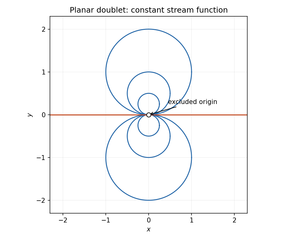
The complex potential of a two-dimensional potential flow is $w=\varphi +i\psi$, soFor $\mu \ne 0$, a nonzero level $\psi =c$ isThus the streamlines are circles tangent to the horizontal axis at the excluded singular origin, with centers on the vertical axis. Each circle has the origin removed. The zero level is the horizontal axis without the origin, whose positive and negative rays are separate streamlines. Since $w^{\prime }=-\mu /z^2$ is nonzero away from the origin, no other stagnation points intervene. For $\mu =0$ the flow vanishes everywhere off the origin, so the circle description is replaced by the degenerate zero-velocity field.

For a twice continuously differentiable stream function, equality of mixed derivatives givesThis is the incompressible flow condition in two dimensions. A streamline is a curve whose tangent at each regular point is parallel to the instantaneous velocity field. Parameterize it by ${\gamma }^{\prime }(s)=c(s)(u,v)$. The chain rule yieldsTherefore the stream function is constant on each streamline. This proof includes arbitrary regular parametrizations; at a stagnation point the velocity vanishes and the usual tangent direction is not determined.

The constraint set $S^1\times S^2$ is compact, so the continuous objective attains a maximum and minimum. The two constraint gradients are nonzero and supported on separate coordinates, so they are linearly independent everywhere on it. The Lagrange multiplier equations areBoth positive and negative values occur. At a maximizing or minimizing point the objective is therefore nonzero, so $x_1\ne 0$, $y_2-y_3\ne 0$, and both $\lambda ,\mu$ are nonzero. The equations imply $x_2=0$, $y_1=0$, and $y_3=-y_2$. The constraints then give $x_1=\pm 1$, $y_2=\pm 1/\sqrt{2}$.

Consequently, writing $s=\pm 1$, the complete list of extrema isFor an independent global check, Cauchy-Schwarz inequality gives $|x_1(y_2-y_3)|\le |x_1|\sqrt{2(y_2^2+y_3^2)}\le \sqrt{2}$, with equality exactly at the displayed points.

The rows of the Jacobian matrix $Dg(a)$ are $\nabla g_1(a{)}^T,\dots ,\nabla g_k(a{)}^T$. Rank $k$ means precisely that these $k$ gradients are linearly independent. The Lagrange multiplier condition is that real numbers ${\lambda }_1,\dots ,{\lambda }_k$ exist withGeometrically, $\nabla f(a)$ is perpendicular to the tangent space of the constraint level set, whose tangent vectors form $\ker Dg(a)$. The full-rank hypothesis ensures this level set is a smooth local constraint manifold.

False. In $X=\mathbb{R}$, takeThen $A\cap B=\{2\}$ and $A\cup B=[0,2]$ are connected. Nevertheless $A$ is disconnected: $[0,1)$ and $\{2\}$ are disjoint nonempty relatively open sets partitioning $A$. For instance, intersecting $A$ with $(-1,3/2)$ and $(3/2,3)$ produces this separation. The endpoint missing from $[0,1)$ is supplied by $B$, so the union becomes connected without forcing $A$ itself to be connected.

False. Take $X=\mathbb{R}$ and $A=B=\{0\}$. Both complements are disconnected: their negative and positive halves form a separation. Butis path-connected, hence connected. To see path connectedness directly, move any nonzero point radially to its normalization on the unit circle; join the two normalized points by a circular arc; then reverse the radial path for the second point. Every segment of this path avoids the origin. Thus disconnected coordinate complements do not force a disconnected complement of their product.

True. Suppose $A\cup B=U\bigsqcup V$ were a separation into nonempty relatively open sets. Intersecting with $A$ gives a separation unless all of the connected set $A$ lies on one side; similarly all of $B$ lies on one side. A point of $A\cap B$ forces both to lie on the same side. The other side would then be empty, a contradiction. Hence $A\cup B$ is connected.

A sequence converges to $x\in X$ whenThe phrase convergent sequence requires the limit to belong to the stated metric space; convergence in a larger ambient space alone does not suffice.

In a metric space, a Cauchy sequence has arbitrarily small distances between all sufficiently late terms:This condition compares terms to each other and does not assume that a limit exists in the space.

A real measurable function is Lebesgue integrable precisely when the integral of its absolute value is finite. For every integer $k\ge 1$, on $I_k=[k+1/6,k+5/6]$ one has $|\sin \pi x|\ge 1/2$ and $x\le k+1$. ConsequentlyThe intervals have disjoint interiors. Countable additivity of the nonnegative Lebesgue integral, or the monotone convergence theorem applied to their finite unions, givesThe harmonic series diverges, so the function is not Lebesgue integrable. Cancellation between adjacent oscillations cannot give absolute integrability.

The Gaussian function is continuous and hence Lebesgue measurable. For $|x|\ge 2$, $x^2/2\ge |x|$, and thereforeThe right side has finite Lebesgue integral: its first term has integral 4 and the second is Lebesgue integrable by hypothesis. The comparison principle for the Lebesgue integral says that a measurable nonnegative function dominated by an integrable function has finite integral. Consequently the Gaussian function is Lebesgue integrable.

Since $K$ is an $F$-vector subspace of the finite-dimensional vector space $L$, it has a finite $F$-basis $u_1,\dots ,u_m$. Any finite $F$-spanning set for $L$ also spans $L$ over $K$, so choose a finite $K$-basis $v_1,\dots ,v_r$ of $L$.

Every $\ell \in L$ can be expanded first in the $v_j$ and then in the $u_i$, showing that the products $u_i{v}_j$ span $L$ over $F$. If ${\sum }_{i,j}{c}_{ij}{u}_i{v}_j=0$ with $c_{ij}\in F$, independence of the $v_j$ over $K$ gives ${\sum }_i{c}_{ij}{u}_i=0$ for every $j$; independence of the $u_i$ then gives every $c_{ij}=0$. The products form an $F$-basis, proving the tower law for field extensions:

A field extension $K/F$ is finite when $K$, regarded as a vector space over $F$, has finite dimension. Its degree of a field extension isThus a finite basis $u_1,\dots ,u_m$ means that every $k\in K$ is uniquely expressible as ${\sum }_i{c}_i{u}_i$ with coefficients $c_i\in F$.

There are six statistical degrees of freedom, so the supplied 1% critical value is $q_6=16.81$. Since $42.25>16.81$, reject independence at the 1% significance level. The data give strong evidence of an association between the two consumption classifications in this group of participants.

Pearson's statistic isFor independent observations under the independence null hypothesis, its large-sample null distribution is approximately ${\chi }^2$ with $(4-1)(3-1)=6$ statistical degrees of freedom. The fitted row and column probabilities account for the reduction in statistical degrees of freedom. All expected counts exceed five, so the usual approximation has adequate expected cell sizes here. Reject independence when the statistic exceeds the corresponding upper-tail critical value.

Under independence, the cell probability is the product of its row and column probabilities. Estimate these by the sample proportions. If $R_i,C_j$ are row and column totals and $N$ is the grand total, the fitted expected count isHere the row totals are $123,76,163,90$, the column totals $304,65,83$, and $N=452$. For example $E_{11}=123\cdot 304/452=82.72566\dots$, rounding to 82.73 as printed. The other entries follow identically.

Applying the chain rule to both inverse identities givesFor the unnumbered calculation, the requested point is $f(c,c)$. The Jacobian there isTo apply its inverse to $(1/2,1/2)$, solve $e^c(v_1+v_2)=1/2$, $e^c{v}_1-e^{-c}{v}_2=1/2$. Subtraction gives $v_2=0$, and henceFor precision, the displayed example maps bijectively onto $V=\{(s,t):s>0,t>0,st>1\}$, rather than the entire positive quadrant. Indeed writing $q=e^x$, the equations are $(s-q)(t-q)=1$ with $0<q<\min (s,t)$. This left side decreases continuously from $st$ to zero, giving exactly one $q$ if and only if $st>1$, after which $e^y=s-q$ is unique. Its Jacobian never vanishes, so the inverse is differentiable on $V$. The requested point lies in $V$, making the calculation well-defined.