Let ${\delta }_{xx}{U}_{ij}=(U_{i+1,j}-2U_{ij}+U_{i-1,j})/(\Delta x{)}^2$, and define ${\delta }_{yy}$ analogously. The Crank-Nicolson diffusion scheme isUse $U_{ij}^0=u_0(x_i,y_j)$ and zero values on every boundary node for every time level. This is the theta method with $\theta =1/2$ applied to the spatial finite difference method for the heat equation.

The first characteristic polynomial factors asThe two quadratic roots have product one. Both can lie in the closed unit disk only if both have modulus one, requiring $|\alpha +1|\le 2$. At $\alpha =-3$ the root one is triple and $\beta =0$; at $\alpha =1$ the root minus one is double. Both fail the root condition for a multistep method. In the intervening open interval the two quadratic roots are distinct conjugate unit-modulus roots, different from one. ThusUsing $2\beta =\alpha +3$, the supplied expansion givesThroughout the zero-stable range, $C_3\ne 0$, so every such method has order two. There is a unique higher-order choice:Here $C_3=C_4=0$ and $C_5=1/10\ne 0$, giving exactly order four, with normalized leading truncation error $h^4{y}^{(5)}/120$. But the extra roots are $-5\pm 2\sqrt{6}$, one of modulus greater than one. By the Dahlquist equivalence theorem this consistent but non-zero-stable method is not convergent for arbitrary consistent starting values.

Zero-stability means that perturbations of the starting values of the zero-step recurrence remain bounded by a fixed multiple of their initial size, uniformly as the number of steps tends to infinity on a fixed time interval. In particular solutions of ${\sum }_{j=0}^k{\alpha }_j{e}_{n+j}=0$ obey ${\max }_{n\le N}|e_n|\le C{\max }_{j<k}|e_j|$ with $C$ independent of $N$.

The equivalent root condition for a multistep method isA root outside the unit circle gives exponential growth of a recurrence relation mode; a repeated root on it gives polynomial growth. Repeated roots strictly inside it are harmless because their polynomial factor is dominated by decay.

In the normalization used by the supplied coefficient expansion, the local truncation error of the linear multistep method isThe nonzero sum in the denominator is an explicit hypothesis. Consistency of a numerical method requires $T_n\to 0$ uniformly on a fixed finite time interval for every sufficiently smooth exact solution as $h\to 0$. Equivalently, the two polynomial identities areThese follow by inserting constant and affine functions, or by setting the first two Taylor coefficients $C_0,C_1$ to zero.

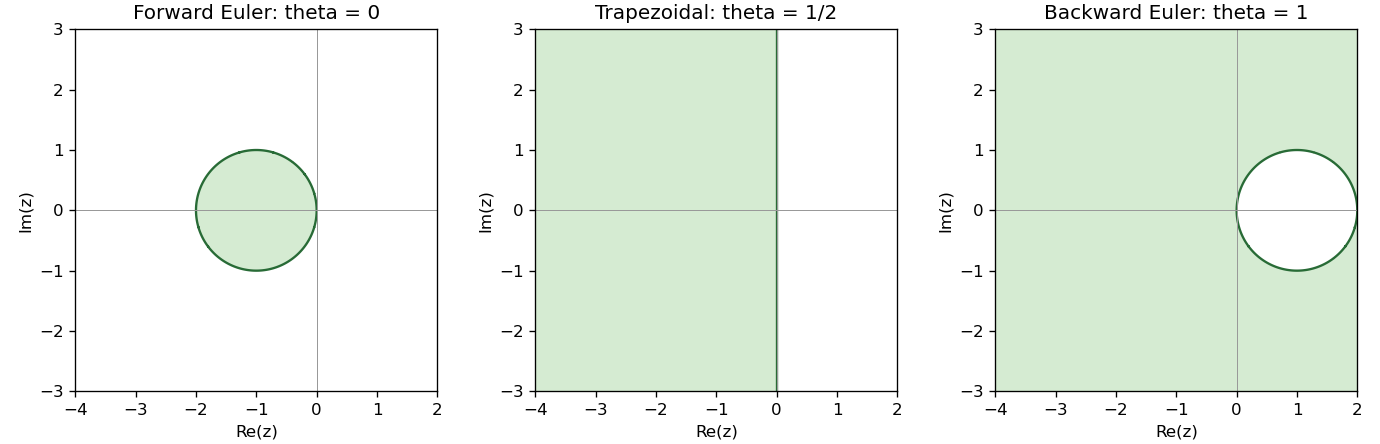
On the Dahlquist test equation, set $z=h\lambda$. The theta method has stability functionWith the decaying-solution convention, its region of absolute stability is $|R(z)|<1$. Writing $z=x+iy$, squaring numerator and denominator givesFor $0\le \theta <1/2$ this is the open disk with centre $-1/(1-2\theta )$ and radius $1/(1-2\theta )$. At $\theta =1/2$ it is the open left half-plane. For $\theta >1/2$ it is the exterior of the closed disk with centre $1/(2\theta -1)$ and radius $1/(2\theta -1)$. The pole $z=1/\theta$, when present, lies outside the stability region.

Every $z$ with $\mathrm{Re}z<0$ satisfies the inequality exactly for $\theta \ge 1/2$. If $\theta <1/2$, sufficiently large negative real $z$ fails it. ThereforeIf absolute stability is instead defined by bounded amplification, the boundary $|R|=1$ is included; this convention does not change the A-stability conclusion for the open left half-plane.

Put $e_n=y(x_n)-y_n$. Subtracting the numerical update from the exact update with its local truncation error givesThe Lipschitz condition in the solution variable and the triangle inequality implyThe assumed positive denominator permits division. With $K=[1+L(1-\theta )h]/(1-L\theta h)$ and $e_0=0$, repeated substitution of this Lipschitz one-step error bound yieldsHere $K>1$ because $L,h>0$, so the displayed geometric series quotient is well defined. For implicit steps, the same condition makes the scalar update map a contraction mapping, ensuring a unique numerical next value.

Use the normalized local truncation errorThe Taylor theorem expansions about $x_n$ areSubstitution gives exactlyThus the theta method has order two exactly for $\theta =1/2$, and otherwise order one, as a statement about the method on a sufficiently smooth class of problems. The leading term vanishes at one half, and a function with nonzero third derivative shows that the next term does not vanish universally. As usual, a uniform order estimate assumes bounded relevant derivatives; mere existence of $y^{\prime \prime \prime }$ on the open interval gives the stated pointwise remainders but not, by itself, a uniform bound. Special exact solutions can of course have zero truncation error even for a first-order method.

The endpoint $\alpha =0$ in the printed nonnegative-parameter hypothesis must be excluded. We first establish the intended result for $\alpha >0$, then describe that endpoint exactly.

Write $X,Y$ for the two directional matrices; they commute because they act on separate tensor-product coordinates. At a limit $V$, the intermediate vector also has a limit $\tilde{V}$. Subtract the two limiting equations in the form that cancels $X\tilde{V}$ and $YV$; this gives $2\alpha (\tilde{V}-V)=0$. Hence $\tilde{V}=V$ for $\alpha >0$. Substitution then gives $(X+Y)V=h^{2}f$, precisely the required discrete equation.

Eliminating the intermediate vector gives the alternating direction implicit iteration matrixThe sine-product basis simultaneously diagonalizes $X,Y$, with eigenvalues $-{\xi }_p$ and $-{\eta }_q$, whereThusFor $\alpha >0$, each factor has modulus strictly less than one. Hence $\rho (G)<1$, proving convergence from every starting vector to the unique discrete solution.

At $\alpha =0$ the two factors are both $-1$, so $G=I$. The forcing terms cancel in the composed iteration as well, and $V^{k+1}=V^k$ for every starting vector. An incorrect initial vector therefore remains incorrect forever, even though the sequence is constant and has a limit. This disproves both the literal fixed-point implication and the claimed general convergence-to-solution assertion at zero; strict positivity of $\alpha$ is the necessary repair.

With zero boundary values eliminated, the diagonal of $L_h$ is $-4I/h^2$. The Jacobi method is thereforewhich averages the four neighboring components. The sine addition identity shows that the supplied product vectors are eigenvectors, withThe discrete sine vectors form a basis, so these are all eigenvalues. Their largest modulus isattained at the lowest and highest sine frequencies. Thus the asymptotic error reduction factor per iteration is $\cos (\pi h)$. If the convergence rate is expressed logarithmically, $R=-\log \rho (J)\sim {\pi }^2{h}^2/2$ as $h\to 0$. A fixed error reduction therefore takes $O(h^{-2})$ Jacobi sweeps. For the special grid $m=2$, $J=0$ and one sweep solves its single interior equation.

The given stencil has nonnegative neighbor weights, zero row sums and a path from every unknown node to the Dirichlet boundary. Thus the discrete maximum principle applies, including at the reflected Neumann edge. The barrier is positive throughout the square.

At an ordinary interior node, central differences differentiate this quadratic exactly, giving $L_h\varphi =2+2=4$. At $x=1$, the reflected horizontal part isand the vertical part is two. Thus $L_h\varphi =4+4/h$ there. Part (c) therefore permitsOn the Dirichlet boundary, the largest barrier value is $4+1/4=17/4$. ConsequentlyThe $O(h)$ truncation error at the Neumann edge is divided by the barrier response $O(h^{-1})$, producing a contribution of order $h^2$. Thus its lower local order does not reduce this global maximum-norm error bound.

The displayed estimate requires a nonnegative barrier. As printed, a counterexample is obtained with two interior nodes, each having row $L_h{v}_p=v_a-v_p$ to one boundary node. Set $e_a=0$, $e_p=1$, and ${\varphi }_a=-1$, ${\varphi }_p=-2$. Both interior rows have $|T_p|=1$ and $L_h{\varphi }_p=1$. Put one node in each of $J_1,J_2$ and take $T=S=d_1=d_2=1$. Then the proposed right-hand side is $-1$ while $E=1$.

For the intended use, suppose ${\varphi }_p\ge 0$ and the stencil has the maximum principle established in part (a). Set $C=\max \{T/d_1,S/d_2\}$. On either subregion,At boundary nodes these functions equal $C{\varphi }_a$. Hencewhich proves the intended discrete elliptic barrier estimateFor a normalized stencil with $L_{h}1=0$ and a sign-changing barrier, shifting it by its minimum gives the valid general replacement $E\le C({\max }_a{\varphi }_a-{\min }_p{\varphi }_p)$. The supplied barrier in part (d) is positive, so the printed estimate applies there without a sign problem.

A diameter-only bound also needs the normalization of a Laplacian stencil, beyond its coefficient signs. For example, a single interior row $L_h{e}_p=\epsilon (e_a-e_p)$ with $e_a=0$ allows $|L_h{e}_p|=1$ and $|e_p|=1/\epsilon$ on a domain of fixed diameter. Thus arbitrary rescaling of the printed coefficients rules out a universal diameter-only estimate.

For the intended normalized Laplacian stencil, assume $L_{h}1=0$ and $L_h\varphi =4$ for ${\varphi }_p=|x_p-x_0{|}^2$, with $x_0\in \Omega$, as holds for the standard two-dimensional central stencil. Let $D=\mathrm{diam}\Omega$. Then $0\le {\varphi }_p\le D^2$. Use the truncation error convention $T_p=L_h{u}_p-f_p$, so $L_h{e}_p=T_p$; reversing the convention does not change the absolute-value argument.

The two functions ${\psi }_p^{\pm }=\pm e_p+(T/4){\varphi }_p$ satisfy $L_h{\psi }^{\pm }\ge -T+T=0$. On the prescribed boundary $e_a=0$, so their maximum boundary values are at most $T{D}^2/4$. Apply the discrete maximum principle from part (a), with its boundary-connectivity assumption. Since $\varphi \ge 0$,This is the standard quadratic-barrier error estimate for a discrete Laplacian. The calculation identifies exactly the additional normalization needed for the bound intended by the question.

The coefficient signs alone do not imply the assertion as printed. Two interior nodes can have rows $L_h{\psi }_1={\psi }_2-{\psi }_1$ and $L_h{\psi }_2={\psi }_1-{\psi }_2$, with a separate boundary node. Taking interior values one and boundary value zero satisfies every stated coefficient inequality and $L_h\psi =0$, but its maximum is not on the boundary. Connectedness of the geometric domain does not ensure connectedness of this stencil graph.

The usual extra assumption is that every interior node has a path of positive stencil coefficients to a prescribed boundary node. Under this assumption let $M\ge 0$ be the global maximum and suppose an interior node $p$ attains it. ThenAll summands are nonpositive, so equality forces ${\psi }_r=M$ at every neighbor with $c_{p,r}>0$. Propagate along a path to the boundary to find a boundary node with value $M$. This proves the discrete maximum principle under boundary-reaching stencil connectivity, and exhibits why the literal hypotheses need that qualification.

Use the fine matrix $A_h$ and right-hand side from part (b), with diagonal $D_h$. Starting from an iterate $v$, take $\nu$ weighted Jacobi smoothing stepsForm the residual $r_h=b_h-A_{h}v$. For coarse interior indices $j=1,\dots ,m/2-1$, use full-weighting restrictionThe prolongation operator matrix $P$ is linear interpolation of a coarse correction: $(Pe{)}_{2j}=e_j$ and $(Pe{)}_{2j+1}=(e_j+e_{j+1})/2$, with zero endpoint corrections. Thus $R=P^T/2$. Choose the Galerkin coarse-grid operator $A_c=R{A}_{h}P$, solve $A_c{e}_c=R{r}_h$ exactly, and correct $v\leftarrow v+P{e}_c$. The entries of $A_h$, $R$ and $P$ above specify every matrix in the cycle. A rediscretized coarse operator is another standard choice if used consistently.

For a nonsingular coarse operator, the fine-grid iteration matrix of this pre-smoothed two-grid cycle isThe purpose of under-relaxation is to damp fine-grid oscillations, leaving smoother error for coarse-grid correction. For the diffusion-dominated one-dimensional operator, $\omega =2/3$ is the usual effective choice; the high-frequency symbol $1-\omega (1-\cos \xi )$ then has modulus at most $1/3$ for $\pi /2\le |\xi |\le \pi$. Coefficients and convection can change the best parameter, so this is a motivated choice rather than a universal optimum. Under the diagonal-dominance condition, the unweighted Jacobi matrix already has norm less than one in the maximum norm, and its convex combination with the identity remains convergent for $0<\omega <1$.

At $x_r=rh$, the central finite difference equations arewith $U_0=\alpha$, $U_m=\beta$. For $f=f(x)$ this is a linear system $A_h{U}_h=b_h$, with row coefficientsThe right-hand side starts from $f(x_r)$ and includes $-a_1\alpha$ in its first entry and $-c_{m-1}\beta$ in its last entry. Under $h\max p<2$, both off-diagonal coefficients are negative, so $|a_r|+|c_r|=2h^{-2}<d_r$. Omitting nonexistent endpoint columns can only reduce this sum. Therefore $A_h$ is strictly diagonally dominant. In particular the linear discrete system is nonsingular.

Introduce $v=u^{\prime }$ and solve the initial-value systemThe unknown initial slope $s$ is the shooting method parameter. Integrate to one and solve the scalar residual equation $R(s)=u(1;s)-\beta =0$, using a secant iteration or a bracketed root finder when suitable data are available.

For a Newton update, integrate the sensitivity equations along the current shot:Then $R^{\prime }(s)=w(1)$ and the update is $s\leftarrow s-R(s)/w(1)$ when this derivative is nonzero. After a root has been found, the corresponding shot satisfies both endpoint conditions. This formulation does not presume that a nonlinear boundary-value problem necessarily has a unique solution.

On nonnegative states the characteristic speed is $f^{\prime }(u)=1+p{u}^{p-1}>0$, so upwind finite difference scheme uses the left spatial difference. With $\lambda =\Delta t/\Delta x$, the conservative upwind finite difference scheme isExplicitly the flux difference is $(U_j^m-U_{j-1}^m)+[(U_j^m{)}^p-(U_{j-1}^m{)}^p]$. Preservation of nonnegativity under the given Courant restriction, proved next, justifies the same left-upwind direction at every step.

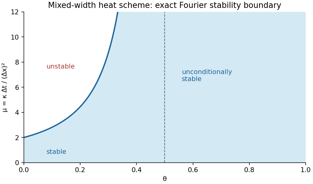
Transforming the spatial shifts and putting $\xi =k\Delta x$ gives the real amplification factorFor $0\le \theta \le 1$ the denominator is at least one, so the implicit step is a bounded Fourier multiplier on ${\ell }^2$. Set $v={\sin }^2(\xi /2)\in [0,1]$ and use ${\sin }^2\xi =4v(1-v)$. The numerator is no greater than the denominator, so $G\le 1$. The other inequality isIf $\theta \ge 1/2$, the bracket is nonpositive and this always holds. If $0\le \theta <1/2$, the concave quadratic has its maximum at $v=(1-2\theta )/[2(1-\theta )]$, with value $(1-2\theta {)}^2/[4(1-\theta )]$. Therefore $|G|\le 1$ precisely under the stated conditionand without a mesh-ratio restriction when $1/2\le \theta \le 1$. The Parseval identity now givesIteration proves stability with constant one. It is conditional for $\theta <1/2$ and unconditional for $\theta \ge 1/2$. The sampled initial data have finite support, hence belong to ${\ell }^2$. This is the Fourier stability threshold for a mixed-width heat scheme.