Put $t=\log x$ and $Y(t)=y(e^t)$. Then $x{y}^{\prime \prime }+y^{\prime }=Y^{\prime \prime }/x$, so the eigenvalue problem reduces toA nonzero Dirichlet eigenfunction therefore has $4+\lambda =n^2$ for an integer $n\ge 1$. The complete family isThe alternatives $4+\lambda \le 0$ give only the zero solution under both endpoint conditions.

The operator itself is self-adjoint with the given unweighted inner product, on the usual regular Dirichlet domain. Indeed $My=(x{y}^{\prime }{)}^{\prime }+4y/x$, and integration by parts givesfor functions satisfying the endpoint conditions. This is a regular Sturm-Liouville operator with positive leading coefficient $x$, whose Dirichlet realization is self-adjoint. The displayed generalized eigenproblem contains the additional weight $1/x$; its eigenfunctions are accordingly orthogonal with respect to $\int fg/x$, which is separate from the self-adjointness assertion about $M$.

Assume a classical solution $u\in C^2(D)\cap C(\overline{D})$, as needed to interpret the boundary values. At an interior local minimum its Hessian is positive semidefinite, hence $\Delta u\ge 0$. But the equation gives $\Delta u=-e^{-x^2}<0$, a contradiction. Since $D$ is bounded and $u=0$ on its boundary, a nonpositive interior value would either furnish an interior negative minimum or itself be a zero minimum. Thus $\boxed{u>0\text{ in }D}$.

For the upper bound use the barrier $w(x,y)=(1-x^2-y^2)/4$, which satisfies $-\Delta w=1$. Set $z=w-u$. On the boundary $z=w\ge 0$, because the domain lies inside the unit disk, whileThe quadratic perturbation proof of the minimum principle gives $z\ge 0$. The strong minimum principle for elliptic operators makes this strict in the connected interior unless $z$ is constant. Constancy is impossible since $1-e^{-x^2}$ is not identically zero on any open domain. HenceThis last strong-principle step handles points with $x=0$, where the comparison forcing itself vanishes. Simple connectedness is not needed for the comparison argument.

With source point $\xi \in D$ and field point $X=(x,y)$, the Dirichlet Green function for the operator $-\Delta$ satisfiesClassically it is harmonic off $\xi$, with the two-dimensional normalization $G(X,\xi )=-(2\pi {)}^{-1}\log |X-\xi |+H(X,\xi )$, where $H$ is regular near the source. Equivalently $-{\lim }_{r\downarrow 0}{\int }_{|X-\xi |=r}{\partial }_{r}Gds=1$. This sign convention gives the representation $u(X)={\int }_{D}G(X,\xi )e^{-{\xi }_1^2}d\xi$.

For $\eta =x/y^{\beta }$ the chain rule gives $u_y=-\beta \eta f^{\prime }/y$, $u_x=y^{-\beta }{f}^{\prime }$ and $(u{u}_x{)}_x=y^{-2\beta }[f{f}^{\prime \prime }+(f^{\prime }{)}^2]$. Multiplication of the equation by $y$ givesA nontrivial scale-invariant balance therefore selects $\boxed{\beta =1/2}$ and yieldsIts left side is the derivative of $f{f}^{\prime }+\eta f/2$. The boundary conditions give $f(0)=1$ and $f^{\prime }(0)=0$, so the integration constant is zero:On the positive branch before the first zero, divide by $f$ and integrate, obtaining $f=1-{\eta }^2/4$. Its first positive zero is ${\eta }_F=2$. HenceA direct check gives $u_y=x^2/(4y^2)$ and $(u{u}_x{)}_x+u/(2y)=x^2/(4y^2)$. The zero extension past this front is also a natural weak compact-support continuation: $u$ is continuous and the degenerate diffusive flux $u{u}_x$ tends to zero at the front. This is a source-driven porous-medium similarity front.

Write the system as $U_x+A(U)U_y=0$ with $U=(u,v{)}^T$ andIts two characteristic speeds are ${\lambda }_{\pm }=v\pm \sqrt{u}$, so it is strictly hyperbolic precisely when $u>0$. At $u=0$ they coincide and the matrix is not diagonalizable; for $u<0$ the speeds are nonreal.

For $u>0$ define $R_{\pm }=v\pm 2\sqrt{u}$ and $D_{\pm }={\partial }_x+(v\pm \sqrt{u}){\partial }_y$. Substitution from the two differential equations givesThereforeThese are the two Riemann invariants; their constancy applies within smooth regions, not across a shock.

Set $F=xp+q^2/4+u-1$. Parametrize the data by $x_0=s$, $y_0=0$, $u_0=1-s^2/3$. Tangential differentiation gives $p_0=-2s/3$; substitution into $F=0$ then gives $q_0^2=4s^2$. Thus the data allow two normal-derivative branches, indexed by $\epsilon =\pm 1$, with $q_0=2\epsilon s$. For $s>0$ each branch is non-characteristic; the endpoint $s=0$ is degenerate.

The Charpit's equations reduce to $\dot{x}=x$, $\dot{y}=q/2$, $\dot{p}=-2p$, $\dot{q}=-q$ and $\dot{u}=xp+q^2/2$. Integrating with these initial values givesDirect substitution checks $xp+q^2/4+u-1=0$, and $t=0$ recovers the initial data. The projection onto the $(x,y)$ plane has Jacobian determinantIt first vanishes at $t=\log 2$. These points form the characteristic caustic $y=\epsilon x/4$, $0<x\le 2$; a single classical solution cannot in general be continued through the fold by treating all projected characteristic curves as a graph.

For a precise description put $r=\epsilon y$. On the chart containing the initial curve and lying before the fold, $t<\log 2$, elimination givesThe plus square-root is forced by $s/x>1/2$, rather than a free second choice. The conditions $0<s\le 1$ give the complete unfolded chartInterior points of the domain have strict inequality at the boundary generated by $s=1$ as well. The other boundary is the characteristic caustic; the original endpoint $s=0$ contributes no open chart. On the portion obtained by following characteristics forward from the data, $0\le t<\log 2$, the region is more specificallyThe $s=1$ boundary is $y=\epsilon (1-1/x)$ and meets the characteristic caustic at $(2,\epsilon /2)$. Negative characteristic times give the continuation across the initial segment into the opposite half-plane. Each sign branch is a distinct local solution; the initial values alone do not select one of them.

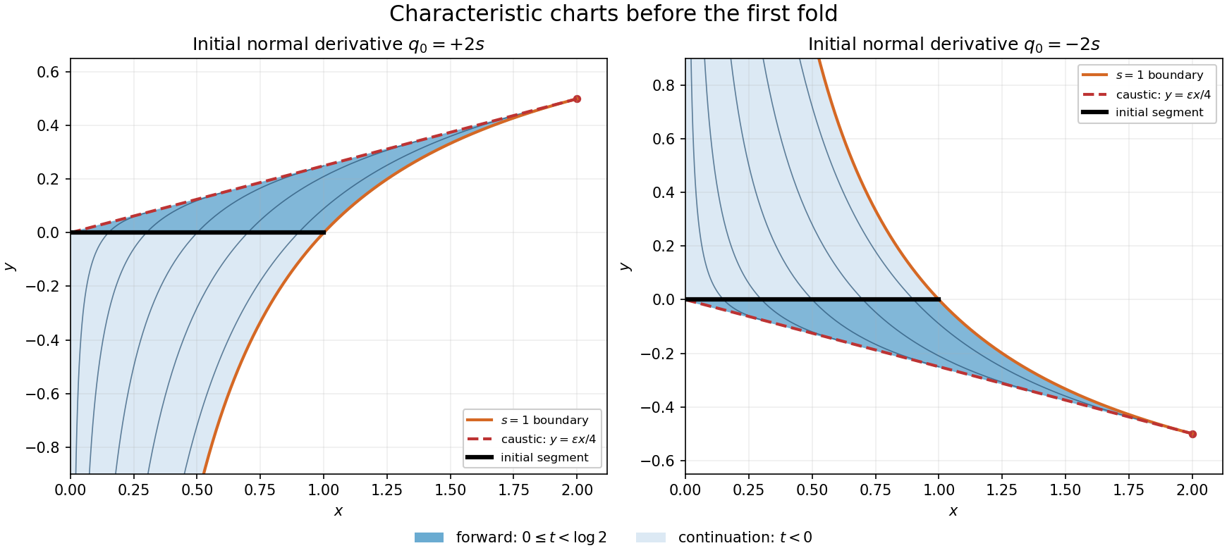
The solid shading follows $t\ge 0$; the lighter shading shows the same smooth chart at $t<0$. Reflected panels correspond to the two allowed signs of the initial normal derivative. Beyond the dashed characteristic caustic the characteristic parametrization no longer gives this smooth graph.

Use the initial-curve parameter $s$ and a characteristic parameter $t$. Charpit's equations areAt $t=0$ prescribe $x=x_0(s)$, $y=y_0(s)$ and $u=u_0(s)$. The two initial derivatives $p_0,q_0$ must satisfyThe second equation is the chain rule along the initial curve. For the usual local Cauchy construction also require the non-characteristic condition $x_0^{\prime }{F}_q-y_0^{\prime }{F}_p\ne 0$. It ensures both local determination of an allowed branch of $p_0,q_0$ and local inversion of the projected characteristic coordinates.

Along a characteristic, the chain rule and the five equations giveSince $F=0$ initially, $\boxed{F\equiv 0}$ along each constructed curve. With the contact compatibility $du=pdx+qdy$ propagated by this system, an invertible characteristic chart reconstructs $p=u_x,q=u_y$ and hence a local classical solution.

Assume first that $n\ge m$. Substituting Rodrigues' formula for $L_n$ givesHere integration by parts was performed $n$ times. Each boundary term vanishes: at infinity a polynomial times $e^{-x}$ tends to zero; at zero every derivative of $x^n{e}^{-x}$ of order less than $n$ vanishes. If $n>m$, the derivative $L_m^{(n)}$ is zero, proving orthogonality. The case $m>n$ follows by exchanging the two factors.

For $m=n$, the leading coefficient found above gives $L_n^{(n)}=(-1{)}^n$. ThereforeThe same conclusion includes $n=0$ directly. Thus the full Laguerre orthonormality relation is

Substitute $y={\sum }_{k\ge 0}{a}_k{x}^k$ and compare the coefficient of $x^k$. The two derivative terms give $(k+1{)}^2{a}_{k+1}$, while the remaining terms give $(n-k)a_k$. ThusIterating the recurrence givesIndeed the recurrence first vanishes at $k=n$ and then remains zero. Consequently the Laguerre polynomial iswith exact degree $n$ and leading coefficient $(-1{)}^n/n!$. This is the regular power-series branch normalized at zero; the second branch at the repeated indicial root is not an additional analytic solution with this normalization.

Normalize the Laguerre differential equation as $y^{\prime \prime }+P(x)y^{\prime }+Q(x)y=0$, where $P(x)=1/x-1$ and $Q(x)=n/x$. At $x=0$, the products $xP=1-x$ and $x^{2}Q=nx$ are analytic. Thus zero is a regular singular point, with indicial equationAt $x=1$ the coefficients $P,Q$ are analytic, so it is an ordinary point. No singular-point indicial equation is needed there.

For infinity put $z=1/x$ and $Y(z)=y(1/z)$. Then the equation becomesAt $z=0$, the coefficient $z(z^{-1}+z^{-2})=1+1/z$ is not analytic. Therefore infinity is an irregular singular point, including when $n=0$. A terminating polynomial solution does not change the classification of the differential equation.